Creating a list based on cell contents

[scotthannaford1973]

Hi all

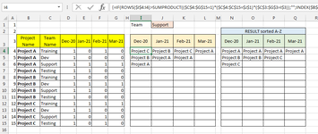
okay hope you can help here... A3:G15 shows a list of projects and project teams; if they are involved in a project in a particular month, there is a 1 beside the team name for that month; if not, there is a 0.

Cell J1 is a drop-down where I can specify the team; what I'd like is that below each month (I3:L3) to list all of the projects where the Team's involvement = 1 and its a dynamic list depending on what's in J1

for example, in J (Jan-21), with Support selected, there would be a list of Project A and Project B

No idea how to do this, so any pointers gratefully received!

A	B	C	D	E	F	G	H	I	J	K	L
1								Team name	Support
2
3	Project Name	Team Name	Dec-20	Jan-21	Feb-21	Mar-21		Dec-20	Jan-21	Feb-21	Mar-21
4	Project A	Training	1	0	1	0
5	Project A	Dev	1	0	0	0
6	Project A	Support	1	1	1	1
7	Project A	Testing	1	1	0	0
8	Project B	Training	1	0	0	0
9	Project B	Dev	1	1	1	1
10	Project B	Support	1	1	0	0
11	Project B	Testing	1	0	0	0
12	Project C	Training	1	1	1	1
13	Project C	Dev	1	1	0	0
14	Project C	Support	1	0	1	0
15	Project C	Testing	1	0	1	0

 

[Fluff]

What version of Excel are you using?
Please update your account details to show this, as it affects which functions you can use.

 

[sandy666]

is that what you want?

Team Name	Support
Attribute	Jan-21
Project Name
Project A
Project B

 

[JLGWhiz]

I am not sure about the column numbers. I tried to guess whether you actually use column A for line numbers or if your project names are in column A. I wrote the code assuming the project names were in column A. If I guesses wrong the code fails and will need to be tweaked.

Private Sub Worksheet_Change(ByVal Target As Range)
If Target.Cells.Count > 1 Then Exit Sub
Application.EnableEvents = False
Dim c As Range, i As Long
    If Target.Address = "$J$1" Then
        For Each c In Range("B4", Cells(Rows.Count, 2).End(xlUp))
            If c.Value = Target.Value Then
                For i = 3 To 6
                    If Cells(c.Row, i) = 1 Then
                        Cells(c.Row, i + 5) = c.Offset(, -1).Value
                    End If
                Next
            End If
        Next
    End If
Application.EnableEvents = True
End Sub

 

[JLGWhiz]

this is the results using the code in post# 4.

Discussions.xlsm
	A	B	C	D	E	F	G	H	I	J	K
1								Team name		Training
2
3	Project Name	Team Name	20-Dec	21-Jan	21-Feb	21-Mar		20-Dec	21-Jan	21-Feb	21-Mar
4	Project A	Training	1	0	1	0		Project A		Project A
5	Project A	Dev	1	0	0	0
6	Project A	Support	1	1	1	1
7	Project A	Testing	1	1	0	0
8	Project B	Training	1	0	0	0		Project B
9	Project B	Dev	1	1	1	1
10	Project B	Support	1	1	0	0
11	Project B	Testing	1	0	0	0
12	Project C	Training	1	1	1	1		Project C	Project C	Project C	Project C
13	Project C	Dev	1	1	0	0
14	Project C	Support	1	0	1	0
15	Project C	Testing	1	0	1	0
Sheet1

 

[sandy666]

or

Team Name	Support
	Attribute
	Dec-20	Feb-21	Jan-21	Mar-21
Team	Project A, Project B, Project C	Project A, Project C	Project A, Project B	Project A

 

[navic]

Try
In 'I4' cell ARRAY formula below (finshed with Ctrl+Shift+Enter), copy across
Sorted Z-A

=IF(ROWS($I$4:I4)>SUMPRODUCT(($C$4:$G$15=1)*($C$4:$C$15=$J$1)*($C$3:$G$3=I$3)),"",INDEX($B$4:$B$15,SUMPRODUCT(LARGE(($C$4:$G$15=1)*($C$4:$C$15=$J$1)*($C$3:$G$3=I$3)*(ROW($C$4:$G$15)-ROW(C$4:G$4)+1),ROWS($I$4:I4)))))

Then Sorted A-Z
In 'N4' cell ARRAY formula below (finshed with Ctrl+Shift+Enter), copy across

=IFERROR(INDEX(I$4:I$15,LARGE(IF(I$4:I$15<>"",ROW(I$4:I$15)-MIN(ROW(I$4:I$15))+1,""),ROWS(N$3:N3))),"")

 

[Fluff]

Two other options depending of your version

+Fluff v2.xlsm
	A	B	C	D	E	F	G	H	I	J	K	L
1									Team name	Support
2
3		Project Name	Team Name	Dec-20	Jan-21	Feb-21	Mar-21		Dec-20	Jan-21	Feb-21	Mar-21
4		Project A	Training	1	0	1	0		Project A	Project A	Project A	Project A
5		Project A	Dev	1	0	0	0		Project B	Project B	Project C
6		Project A	Support	1	1	1	1		Project C
7		Project A	Testing	1	1	0	0
8		Project B	Training	1	0	0	0
9		Project B	Dev	1	1	1	1		Project A	Project A	Project A	Project A
10		Project B	Support	1	1	0	0		Project B	Project B	Project C
11		Project B	Testing	1	0	0	0		Project C
12		Project C	Training	1	1	1	1
13		Project C	Dev	1	1	0	0
14		Project C	Support	1	0	1	0
15		Project C	Testing	1	0	1	0
16
Main

Cell Formulas
Range	Formula
I4:I6,L4,J4:K5	I4	=FILTER($B$4:$B$15,($C$4:$C$15=$J$1)*(FILTER($D$4:$G$15,$D$3:$G$3=I3)=1))
I9:L12	I9	=IFERROR(INDEX($B$4:$B$15,AGGREGATE(15,6,(ROW($B$4:$B$15)-ROW($B$4)+1)/($C$4:$C$15=$J$1)/($D$3:$G$3=I$3)/($D$4:$G$15=1),ROWS(I$9:I9))),"")
Dynamic array formulas.

 

[scotthannaford1973]

Try
In 'I4' cell ARRAY formula below (finshed with Ctrl+Shift+Enter), copy across
Sorted Z-A

=IF(ROWS($I$4:I4)>SUMPRODUCT(($C$4:$G$15=1)*($C$4:$C$15=$J$1)*($C$3:$G$3=I$3)),"",INDEX($B$4:$B$15,SUMPRODUCT(LARGE(($C$4:$G$15=1)*($C$4:$C$15=$J$1)*($C$3:$G$3=I$3)*(ROW($C$4:$G$15)-ROW(C$4:G$4)+1),ROWS($I$4:I4)))))

Then Sorted A-Z
In 'N4' cell ARRAY formula below (finshed with Ctrl+Shift+Enter), copy across

=IFERROR(INDEX(I$4:I$15,LARGE(IF(I$4:I$15<>"",ROW(I$4:I$15)-MIN(ROW(I$4:I$15))+1,""),ROWS(N$3:N3))),"")

thanks - that works like a dream

Try
In 'I4' cell ARRAY formula below (finshed with Ctrl+Shift+Enter), copy across
Sorted Z-A

=IF(ROWS($I$4:I4)>SUMPRODUCT(($C$4:$G$15=1)*($C$4:$C$15=$J$1)*($C$3:$G$3=I$3)),"",INDEX($B$4:$B$15,SUMPRODUCT(LARGE(($C$4:$G$15=1)*($C$4:$C$15=$J$1)*($C$3:$G$3=I$3)*(ROW($C$4:$G$15)-ROW(C$4:G$4)+1),ROWS($I$4:I4)))))

Then Sorted A-Z
In 'N4' cell ARRAY formula below (finshed with Ctrl+Shift+Enter), copy across

=IFERROR(INDEX(I$4:I$15,LARGE(IF(I$4:I$15<>"",ROW(I$4:I$15)-MIN(ROW(I$4:I$15))+1,""),ROWS(N$3:N3))),"")

 

[scotthannaford1973]

thanks all - some great suggestions there - works like a dream

=IF(ROWS($I$4:I4)>SUMPRODUCT(($C$4:$G$15=1)*($C$4:$C$15=$J$1)*($C$3:$G$3=I$3)),"",INDEX($B$4:$B$15,SUMPRODUCT(LARGE(($C$4:$G$15=1)*($C$4:$C$15=$J$1)*($C$3:$G$3=I$3)*(ROW($C$4:$G$15)-ROW(C$4:G$4)+1),ROWS($I$4:I4)))))