Cross search matching data

Robinazer

New Member
Joined
Feb 18, 2021
Messages
6
Office Version
  1. 365
Platform
  1. Windows
My employer asked me to automate the duplicate positioned items in excel. Our company works with 20.000+ items and the stock in all of the locations is automatically updated each day. When new items are moved by a branch, they often forget to remove the replaced item out of our database. The location X, X, X, X (rack, shelve, spot, little compartment) now has 2 Items in the database but only 1 in reality.

If for example item D replaces item B at location 1, 1, 1, 1 and they add D in the database but forget to remove B, we see the following


ItemBranchLocation nr 1Location nr 2Location nr 3Location nr 4
A32751532
B32751111
C32751312
D32751111


With only 4 items, it is easy to see that B and D share the same position in the same branch which is an obvious mistake. With over 20.000 items, you have to manually look at each location at each branch which normally takes about 4 to 5 days.


The same X.X.X.X. values exist in different branches. the same products are in in different branches. There are around 80 branches. Each branch has up to 9 * 9 * 9 * 9 = 6.561 items (where as 9 is the highest number for a location). Here a more detailed and correct example of our database:


BranchItemLocation 1Location 2Location 3Location 4
300033871111
300033901112
300033881113
300033921114
300033451115
323033781111
323033361112
323033691113
327533871111
327533361112
327533501113
327533591111
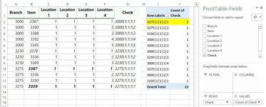
As you can see, the location 1, 1, 1, 1 is in every branch which is okay, but since it is twice in branch 3275, this is a problem.

Is there a way to make a calculation/formula in excel so that I only have to upload the generated XML database and the calculation gives me the duplicate items and their locations automatically?
 

Excel Facts

Copy formula down without changing references
If you have =SUM(F2:F49) in F50; type Alt+' in F51 to copy =SUM(F2:F49) to F51, leaving the formula in edit mode. Change SUM to COUNT.
Create a check string column ... concatenate branch with all the locations into one string ... a PivotTable will show duplicates in 2 minutes.
 
Upvote 0
Welcome to the MrExcel board!

It isn't clear to me exactly what you want presented. Is it something like this?

21 02 19.xlsm
ABCDEFG
1BranchItemLocation 1Location 2Location 3Location 4
2300033871111 
3300033901112 
4300033881113 
5300033921114 
6300033451115 
7323033781111 
8323033361112 
9323033691113 
10327533871111Dupe
11327533361112 
12327533501113 
13327533591111Dupe
Sheet2 (2)
Cell Formulas
RangeFormula
G2:G13G2=IF(COUNTIFS(A$2:A$13,A2,C$2:C$13,C2,D$2:D$13,D2,E$2:E$13,E2,F$2:F$13,F2)>1,"Dupe","")


If not can you post what you would want returned based on your second sample data above?

Also, is it possible to have 3 or more rows with the same Branch/Location details? If so, please include an example like that in new sample data and expected results.
 
Upvote 0
Here is what I was suggesting as a solution: (sorted, Large to Smallest ... all the clashes will appear at the top)
 

Attachments

  • PT_Check_col.JPG
    PT_Check_col.JPG
    89.2 KB · Views: 8
Upvote 0
Create a check string column ... concatenate branch with all the locations into one string ... a PivotTable will show duplicates in 2 minutes.
It was solved by using a Countifs function.
=COUNTIFS(A:A;A2;G:G;G2;H:H;H2;I:I;I2;J:J;J2)>1
Your solution will probably be better but since I'm a total excel noob this will do. Thanks for your reply ^^
 
Upvote 0
Welcome to the MrExcel board!

It isn't clear to me exactly what you want presented. Is it something like this?

21 02 19.xlsm
ABCDEFG
1BranchItemLocation 1Location 2Location 3Location 4
2300033871111 
3300033901112 
4300033881113 
5300033921114 
6300033451115 
7323033781111 
8323033361112 
9323033691113 
10327533871111Dupe
11327533361112 
12327533501113 
13327533591111Dupe
Sheet2 (2)
Cell Formulas
RangeFormula
G2:G13G2=IF(COUNTIFS(A$2:A$13,A2,C$2:C$13,C2,D$2:D$13,D2,E$2:E$13,E2,F$2:F$13,F2)>1,"Dupe","")


If not can you post what you would want returned based on your second sample data above?

Also, is it possible to have 3 or more rows with the same Branch/Location details? If so, please include an example like that in new sample data and expected results.
It was solved by using a Countifs function.
=COUNTIFS(A:A;A2;G:G;G2;H:H;H2;I:I;I2;J:J;J2)>1
I used your example and simplified it a bit. Thanks for your reply ^^
 
Upvote 0
Here is what I was suggesting as a solution: (sorted, Large to Smallest ... all the clashes will appear at the top)
It was solved by using a Countifs function.
=COUNTIFS(A:A;A2;G:G;G2;H:H;H2;I:I;I2;J:J;J2)>1
Since the item can be faulty placed at every location, your example would still take a lot of time. I'd have to check each of the 6.500+ unique locations.
Thanks for your reply ^^
 
Upvote 0
It was solved by using a Countifs function.
=COUNTIFS(A:A;A2;G:G;G2;H:H;H2;I:I;I2;J:J;J2)>1
Since the item can be faulty placed at every location, your example would still take a lot of time. I'd have to check each of the 6.500+ unique locations.
Thanks for your reply ^^
I don't believe you actually understand what I did. Any dup will be greater than 1 in the PivotTable ... and sorting the results largest to smallest shows them all at the top of the list.
 
Upvote 0

Forum statistics

Threads
1,214,785
Messages
6,121,543
Members
449,038
Latest member
Guest1337

We've detected that you are using an adblocker.

We have a great community of people providing Excel help here, but the hosting costs are enormous. You can help keep this site running by allowing ads on MrExcel.com.
Allow Ads at MrExcel

Which adblocker are you using?

Disable AdBlock

Follow these easy steps to disable AdBlock

1)Click on the icon in the browser’s toolbar.
2)Click on the icon in the browser’s toolbar.
2)Click on the "Pause on this site" option.
Go back

Disable AdBlock Plus

Follow these easy steps to disable AdBlock Plus

1)Click on the icon in the browser’s toolbar.
2)Click on the toggle to disable it for "mrexcel.com".
Go back

Disable uBlock Origin

Follow these easy steps to disable uBlock Origin

1)Click on the icon in the browser’s toolbar.
2)Click on the "Power" button.
3)Click on the "Refresh" button.
Go back

Disable uBlock

Follow these easy steps to disable uBlock

1)Click on the icon in the browser’s toolbar.
2)Click on the "Power" button.
3)Click on the "Refresh" button.
Go back
Back
Top