CSV data with fields in different order on each row

[ASB21]

I have a CSV dataset that contains a series of rows each with a number of different data fields populated by having selecting from a series of pre-defined options. The name of each option across all the data fields is unique, so for example no two fields would contain "high" as an option but each one would have a name specific to that field.

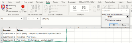
The problems I have are that the same field is not always in the same position in every row, not every field is always populated in each row and there are spaces between the delimiter in the dataset and each data point. For example something like this (but with many more data fields):

Good quality | Low price | Good service | Poor location
High price | Poor service
Poor service | Medium price | Medium quality

I would like to format the dataset so that I can see each field in the same column on every row in a table (and show a blank if no option has been selected for that field in that row). I think I have a potential solution but it's not a good one - to do Text to Columns and then do a series of If / Countif statements in each column of a new table to get the data into the format I want, for example in the "Quality" column of the new table row 2 would look like:

=IF(COUNTIF($A2:$D2,"Good quality ")>0,"Good quality",IF(COUNTIF($A2:$D2,"Medium quality ")>0,"Medium quality",IF(COUNTIF($A2:$D2,"Poor quality ")>0,"Poor quality","")))

However I suppose I'd also need to add in the options where there was also a space at the beginning of the name (where it wasn't the first field in a row) and in any case for the size of the dataset I think it would just take too long to set up and assume there must be a better way. So I was hoping someone could help and suggest something better please? Many thanks in advance!

 

[Kerryx]

An example of the dataset ( hiding any sensitive data) would be of assistance, please use the XL2BB addon to give us something to work with

 

[ASB21]

An example of the dataset ( hiding any sensitive data) would be of assistance, please use the XL2BB addon to give us something to work with

Hi, thanks - hopefully I've done this correctly. It's the yellow cells in the second table I'm looking to populate with formulae that automatically results in the third table.

Excel Example.xlsx
	A	B	C	D	E	F	G	H	I	J	K	L	M	N
1	Original data			Table to be populated automatically						Required outcome once automatically populated
2
3	Company	Ratings		Company	Location	Price	Service	Quality		Company	Location	Price	Service	Quality
4	Supermarket A	Good quality | Low price | Good service | Poor location		Supermarket A						Supermarket A	Poor location	Low price	Good service	Good quality
5	Supermarket B	High price | Poor service		Supermarket B						Supermarket B		High price	Poor service
6	Supermarket C	Poor service | Medium price | Medium quality		Supermarket C						Supermarket C		Medium price	Poor service	Medium quality
Example

 

[Kerryx]

Could just load to Power query

let
    Source = Excel.CurrentWorkbook(){[Name="Table1"]}[Content],
    #"Changed Type" = Table.TransformColumnTypes(Source,{{"Company", type text}, {"Ratings", type text}}),
    #"Split Column by Delimiter" = Table.SplitColumn(#"Changed Type", "Ratings", Splitter.SplitTextByDelimiter("|", QuoteStyle.Csv), {"Ratings.1", "Ratings.2", "Ratings.3", "Ratings.4"}),
    #"Replaced Value" = Table.ReplaceValue(#"Split Column by Delimiter",null,"",Replacer.ReplaceValue,{"Ratings.1", "Ratings.2", "Ratings.3", "Ratings.4"}),
    #"Added Custom" = Table.AddColumn(#"Replaced Value", "Location", each if Text.Contains([Ratings.1], "location") then [Ratings.1] else if Text.Contains([Ratings.2], "location") then [Ratings.2] else if Text.Contains([Ratings.3], "location") then [Ratings.3] else if Text.Contains([Ratings.4], "location") then [Ratings.4] else ""),
    #"Added Custom1" = Table.AddColumn(#"Added Custom", "Price", each if Text.Contains([Ratings.1], "price") then [Ratings.1] else if Text.Contains([Ratings.2], "price") then [Ratings.2] else if Text.Contains([Ratings.3], "price") then [Ratings.3] else if Text.Contains([Ratings.4], "price") then [Ratings.4] else ""),
    #"Added Custom2" = Table.AddColumn(#"Added Custom1", "Service", each if Text.Contains([Ratings.1], "service") then [Ratings.1] else if Text.Contains([Ratings.2], "service") then [Ratings.2] else if Text.Contains([Ratings.3], "service") then [Ratings.3] else if Text.Contains([Ratings.4], "service") then [Ratings.4] else ""),
    #"Added Custom3" = Table.AddColumn(#"Added Custom2", "Quality", each if Text.Contains([Ratings.1], "quality") then [Ratings.1] else if Text.Contains([Ratings.2], "quality") then [Ratings.2] else if Text.Contains([Ratings.3], "quality") then [Ratings.3] else if Text.Contains([Ratings.4], "quality") then [Ratings.4] else ""),
    #"Removed Columns" = Table.RemoveColumns(#"Added Custom3",{"Ratings.1", "Ratings.2", "Ratings.3", "Ratings.4"}),
    #"Trimmed Text" = Table.TransformColumns(#"Removed Columns",{{"Location", Text.Trim, type text}, {"Price", Text.Trim, type text}, {"Service", Text.Trim, type text}, {"Quality", Text.Trim, type text}})
 
in
    #"Trimmed Text"

 

[ASB21]

Could just load to Power query

let
    Source = Excel.CurrentWorkbook(){[Name="Table1"]}[Content],
    #"Changed Type" = Table.TransformColumnTypes(Source,{{"Company", type text}, {"Ratings", type text}}),
    #"Split Column by Delimiter" = Table.SplitColumn(#"Changed Type", "Ratings", Splitter.SplitTextByDelimiter("|", QuoteStyle.Csv), {"Ratings.1", "Ratings.2", "Ratings.3", "Ratings.4"}),
    #"Replaced Value" = Table.ReplaceValue(#"Split Column by Delimiter",null,"",Replacer.ReplaceValue,{"Ratings.1", "Ratings.2", "Ratings.3", "Ratings.4"}),
    #"Added Custom" = Table.AddColumn(#"Replaced Value", "Location", each if Text.Contains([Ratings.1], "location") then [Ratings.1] else if Text.Contains([Ratings.2], "location") then [Ratings.2] else if Text.Contains([Ratings.3], "location") then [Ratings.3] else if Text.Contains([Ratings.4], "location") then [Ratings.4] else ""),
    #"Added Custom1" = Table.AddColumn(#"Added Custom", "Price", each if Text.Contains([Ratings.1], "price") then [Ratings.1] else if Text.Contains([Ratings.2], "price") then [Ratings.2] else if Text.Contains([Ratings.3], "price") then [Ratings.3] else if Text.Contains([Ratings.4], "price") then [Ratings.4] else ""),
    #"Added Custom2" = Table.AddColumn(#"Added Custom1", "Service", each if Text.Contains([Ratings.1], "service") then [Ratings.1] else if Text.Contains([Ratings.2], "service") then [Ratings.2] else if Text.Contains([Ratings.3], "service") then [Ratings.3] else if Text.Contains([Ratings.4], "service") then [Ratings.4] else ""),
    #"Added Custom3" = Table.AddColumn(#"Added Custom2", "Quality", each if Text.Contains([Ratings.1], "quality") then [Ratings.1] else if Text.Contains([Ratings.2], "quality") then [Ratings.2] else if Text.Contains([Ratings.3], "quality") then [Ratings.3] else if Text.Contains([Ratings.4], "quality") then [Ratings.4] else ""),
    #"Removed Columns" = Table.RemoveColumns(#"Added Custom3",{"Ratings.1", "Ratings.2", "Ratings.3", "Ratings.4"}),
    #"Trimmed Text" = Table.TransformColumns(#"Removed Columns",{{"Location", Text.Trim, type text}, {"Price", Text.Trim, type text}, {"Service", Text.Trim, type text}, {"Quality", Text.Trim, type text}})
 
in
    #"Trimmed Text"

View attachment 75060

Amazing, thank you - I've never used Power Query before but will give it a go. Really appreciate your help!

 

[ASB21]

Could just load to Power query

let
    Source = Excel.CurrentWorkbook(){[Name="Table1"]}[Content],
    #"Changed Type" = Table.TransformColumnTypes(Source,{{"Company", type text}, {"Ratings", type text}}),
    #"Split Column by Delimiter" = Table.SplitColumn(#"Changed Type", "Ratings", Splitter.SplitTextByDelimiter("|", QuoteStyle.Csv), {"Ratings.1", "Ratings.2", "Ratings.3", "Ratings.4"}),
    #"Replaced Value" = Table.ReplaceValue(#"Split Column by Delimiter",null,"",Replacer.ReplaceValue,{"Ratings.1", "Ratings.2", "Ratings.3", "Ratings.4"}),
    #"Added Custom" = Table.AddColumn(#"Replaced Value", "Location", each if Text.Contains([Ratings.1], "location") then [Ratings.1] else if Text.Contains([Ratings.2], "location") then [Ratings.2] else if Text.Contains([Ratings.3], "location") then [Ratings.3] else if Text.Contains([Ratings.4], "location") then [Ratings.4] else ""),
    #"Added Custom1" = Table.AddColumn(#"Added Custom", "Price", each if Text.Contains([Ratings.1], "price") then [Ratings.1] else if Text.Contains([Ratings.2], "price") then [Ratings.2] else if Text.Contains([Ratings.3], "price") then [Ratings.3] else if Text.Contains([Ratings.4], "price") then [Ratings.4] else ""),
    #"Added Custom2" = Table.AddColumn(#"Added Custom1", "Service", each if Text.Contains([Ratings.1], "service") then [Ratings.1] else if Text.Contains([Ratings.2], "service") then [Ratings.2] else if Text.Contains([Ratings.3], "service") then [Ratings.3] else if Text.Contains([Ratings.4], "service") then [Ratings.4] else ""),
    #"Added Custom3" = Table.AddColumn(#"Added Custom2", "Quality", each if Text.Contains([Ratings.1], "quality") then [Ratings.1] else if Text.Contains([Ratings.2], "quality") then [Ratings.2] else if Text.Contains([Ratings.3], "quality") then [Ratings.3] else if Text.Contains([Ratings.4], "quality") then [Ratings.4] else ""),
    #"Removed Columns" = Table.RemoveColumns(#"Added Custom3",{"Ratings.1", "Ratings.2", "Ratings.3", "Ratings.4"}),
    #"Trimmed Text" = Table.TransformColumns(#"Removed Columns",{{"Location", Text.Trim, type text}, {"Price", Text.Trim, type text}, {"Service", Text.Trim, type text}, {"Quality", Text.Trim, type text}})
 
in
    #"Trimmed Text"

View attachment 75060

Hi, I've given it a go today and struggling a bit - I've managed to follow a YouTube tutorial to create a basic Power Query and been able to do the Split Column by Delimiter step but struggling to know how to create the rest of the query you've suggested (I can't see anywhere for example just to paste in the text above as you seem to have to do it via "recording" it yourself).

Sorry I'm sure this is all basic stuff but as I'd never used Power Query before can you suggest any articles or videos that would help me get to the level of being able to put what you've suggested into practice please?

 

[Kerryx]

Ok starting with the sorce , assuming like below 2 columns

In power query go to Home tab, select Advanced editor

Here as long as the column names and source table name are the same as above, you can simply delete everything in the advanced editor screen, copy and paste the following into it instead

let
    Source = Excel.CurrentWorkbook(){[Name="Table1"]}[Content],
    #"Changed Type" = Table.TransformColumnTypes(Source,{{"Company", type text}, {"Ratings", type text}}),
    #"Split Column by Delimiter" = Table.SplitColumn(#"Changed Type", "Ratings", Splitter.SplitTextByDelimiter("|", QuoteStyle.Csv), {"Ratings.1", "Ratings.2", "Ratings.3", "Ratings.4"}),
    #"Replaced Value" = Table.ReplaceValue(#"Split Column by Delimiter",null,"",Replacer.ReplaceValue,{"Ratings.1", "Ratings.2", "Ratings.3", "Ratings.4"}),
    #"Added Custom" = Table.AddColumn(#"Replaced Value", "Location", each if Text.Contains([Ratings.1], "location") then [Ratings.1] else if Text.Contains([Ratings.2], "location") then [Ratings.2] else if Text.Contains([Ratings.3], "location") then [Ratings.3] else if Text.Contains([Ratings.4], "location") then [Ratings.4] else ""),
    #"Added Custom1" = Table.AddColumn(#"Added Custom", "Price", each if Text.Contains([Ratings.1], "price") then [Ratings.1] else if Text.Contains([Ratings.2], "price") then [Ratings.2] else if Text.Contains([Ratings.3], "price") then [Ratings.3] else if Text.Contains([Ratings.4], "price") then [Ratings.4] else ""),
    #"Added Custom2" = Table.AddColumn(#"Added Custom1", "Service", each if Text.Contains([Ratings.1], "service") then [Ratings.1] else if Text.Contains([Ratings.2], "service") then [Ratings.2] else if Text.Contains([Ratings.3], "service") then [Ratings.3] else if Text.Contains([Ratings.4], "service") then [Ratings.4] else ""),
    #"Added Custom3" = Table.AddColumn(#"Added Custom2", "Quality", each if Text.Contains([Ratings.1], "quality") then [Ratings.1] else if Text.Contains([Ratings.2], "quality") then [Ratings.2] else if Text.Contains([Ratings.3], "quality") then [Ratings.3] else if Text.Contains([Ratings.4], "quality") then [Ratings.4] else ""),
    #"Removed Columns" = Table.RemoveColumns(#"Added Custom3",{"Ratings.1", "Ratings.2", "Ratings.3", "Ratings.4"}),
    #"Trimmed Text" = Table.TransformColumns(#"Removed Columns",{{"Location", Text.Trim, type text}, {"Price", Text.Trim, type text}, {"Service", Text.Trim, type text}, {"Quality", Text.Trim, type text}})
 
in
    #"Trimmed Text"

So you now have this

Click on Done and you should see the Applied steps appear on the right side of your screen

If you click through these you can see what was done at each step
Next job is to load back into Excel, go to file tab then click on Close and load to

Simply select where you want it to go to on your sheet or new sheet

 

[ASB21]

Ok starting with the sorce , assuming like below 2 columns
View attachment 76043
In power query go to Home tab, select Advanced editor
View attachment 76044
Here as long as the column names and source table name are the same as above, you can simply delete everything in the advanced editor screen, copy and paste the following into it instead

let
    Source = Excel.CurrentWorkbook(){[Name="Table1"]}[Content],
    #"Changed Type" = Table.TransformColumnTypes(Source,{{"Company", type text}, {"Ratings", type text}}),
    #"Split Column by Delimiter" = Table.SplitColumn(#"Changed Type", "Ratings", Splitter.SplitTextByDelimiter("|", QuoteStyle.Csv), {"Ratings.1", "Ratings.2", "Ratings.3", "Ratings.4"}),
    #"Replaced Value" = Table.ReplaceValue(#"Split Column by Delimiter",null,"",Replacer.ReplaceValue,{"Ratings.1", "Ratings.2", "Ratings.3", "Ratings.4"}),
    #"Added Custom" = Table.AddColumn(#"Replaced Value", "Location", each if Text.Contains([Ratings.1], "location") then [Ratings.1] else if Text.Contains([Ratings.2], "location") then [Ratings.2] else if Text.Contains([Ratings.3], "location") then [Ratings.3] else if Text.Contains([Ratings.4], "location") then [Ratings.4] else ""),
    #"Added Custom1" = Table.AddColumn(#"Added Custom", "Price", each if Text.Contains([Ratings.1], "price") then [Ratings.1] else if Text.Contains([Ratings.2], "price") then [Ratings.2] else if Text.Contains([Ratings.3], "price") then [Ratings.3] else if Text.Contains([Ratings.4], "price") then [Ratings.4] else ""),
    #"Added Custom2" = Table.AddColumn(#"Added Custom1", "Service", each if Text.Contains([Ratings.1], "service") then [Ratings.1] else if Text.Contains([Ratings.2], "service") then [Ratings.2] else if Text.Contains([Ratings.3], "service") then [Ratings.3] else if Text.Contains([Ratings.4], "service") then [Ratings.4] else ""),
    #"Added Custom3" = Table.AddColumn(#"Added Custom2", "Quality", each if Text.Contains([Ratings.1], "quality") then [Ratings.1] else if Text.Contains([Ratings.2], "quality") then [Ratings.2] else if Text.Contains([Ratings.3], "quality") then [Ratings.3] else if Text.Contains([Ratings.4], "quality") then [Ratings.4] else ""),
    #"Removed Columns" = Table.RemoveColumns(#"Added Custom3",{"Ratings.1", "Ratings.2", "Ratings.3", "Ratings.4"}),
    #"Trimmed Text" = Table.TransformColumns(#"Removed Columns",{{"Location", Text.Trim, type text}, {"Price", Text.Trim, type text}, {"Service", Text.Trim, type text}, {"Quality", Text.Trim, type text}})
 
in
    #"Trimmed Text"

So you now have this
View attachment 76045
Click on Done and you should see the Applied steps appear on the right side of your screen
View attachment 76047
If you click through these you can see what was done at each step
Next job is to load back into Excel, go to file tab then click on Close and load to
View attachment 76048
Simply select where you want it to go to on your sheet or new sheet

That's brilliant, thank you so much - really grateful to you for spending the time doing that

 

[ASB21]

Ok starting with the sorce , assuming like below 2 columns
View attachment 76043
In power query go to Home tab, select Advanced editor
View attachment 76044
Here as long as the column names and source table name are the same as above, you can simply delete everything in the advanced editor screen, copy and paste the following into it instead

let
    Source = Excel.CurrentWorkbook(){[Name="Table1"]}[Content],
    #"Changed Type" = Table.TransformColumnTypes(Source,{{"Company", type text}, {"Ratings", type text}}),
    #"Split Column by Delimiter" = Table.SplitColumn(#"Changed Type", "Ratings", Splitter.SplitTextByDelimiter("|", QuoteStyle.Csv), {"Ratings.1", "Ratings.2", "Ratings.3", "Ratings.4"}),
    #"Replaced Value" = Table.ReplaceValue(#"Split Column by Delimiter",null,"",Replacer.ReplaceValue,{"Ratings.1", "Ratings.2", "Ratings.3", "Ratings.4"}),
    #"Added Custom" = Table.AddColumn(#"Replaced Value", "Location", each if Text.Contains([Ratings.1], "location") then [Ratings.1] else if Text.Contains([Ratings.2], "location") then [Ratings.2] else if Text.Contains([Ratings.3], "location") then [Ratings.3] else if Text.Contains([Ratings.4], "location") then [Ratings.4] else ""),
    #"Added Custom1" = Table.AddColumn(#"Added Custom", "Price", each if Text.Contains([Ratings.1], "price") then [Ratings.1] else if Text.Contains([Ratings.2], "price") then [Ratings.2] else if Text.Contains([Ratings.3], "price") then [Ratings.3] else if Text.Contains([Ratings.4], "price") then [Ratings.4] else ""),
    #"Added Custom2" = Table.AddColumn(#"Added Custom1", "Service", each if Text.Contains([Ratings.1], "service") then [Ratings.1] else if Text.Contains([Ratings.2], "service") then [Ratings.2] else if Text.Contains([Ratings.3], "service") then [Ratings.3] else if Text.Contains([Ratings.4], "service") then [Ratings.4] else ""),
    #"Added Custom3" = Table.AddColumn(#"Added Custom2", "Quality", each if Text.Contains([Ratings.1], "quality") then [Ratings.1] else if Text.Contains([Ratings.2], "quality") then [Ratings.2] else if Text.Contains([Ratings.3], "quality") then [Ratings.3] else if Text.Contains([Ratings.4], "quality") then [Ratings.4] else ""),
    #"Removed Columns" = Table.RemoveColumns(#"Added Custom3",{"Ratings.1", "Ratings.2", "Ratings.3", "Ratings.4"}),
    #"Trimmed Text" = Table.TransformColumns(#"Removed Columns",{{"Location", Text.Trim, type text}, {"Price", Text.Trim, type text}, {"Service", Text.Trim, type text}, {"Quality", Text.Trim, type text}})
 
in
    #"Trimmed Text"

So you now have this
View attachment 76045
Click on Done and you should see the Applied steps appear on the right side of your screen
View attachment 76047
If you click through these you can see what was done at each step
Next job is to load back into Excel, go to file tab then click on Close and load to
View attachment 76048
Simply select where you want it to go to on your sheet or new sheet

Hi, I have a follow up question on this...

As the real data I'm using has about 50 initial data columns (the equivalent of Ratings.1 to Ratings.4) which I then want to organise into about 60-70 new category columns (the equivalent of Location, Price, Service & Quality) which each have 2-5 potential options (the equivalent of low price, medium price and high price), I'd like to amend the query so that it would be quicker to update if any of the options or categories were to change.

I'm wondering whether I could just have a separate table in another sheet like the one I've created below for this example which has all the categories and potential options that I could then just refer to in the query, and then only need to update the table and not the code each time a category or option changed. Do you have any suggestions of how to modify the query to make this possible please?

Excel Example.xlsx
	A	B	C	D
1	Location	Price	Service	Quality
2	Excellent location	High price	Good service	Good quality
3	Good location	Medium price	Poor service	Medium quality
4	Average location	Low price		Poor quality
5	Poor location
6	Very poor location
Options

Thank you!

 

[ASB21]

Sorry just to add, it's also possible that the options within some categories won't always contain the same word - so perhaps the example below would be better...

Excel Example.xlsx
	A	B	C	D
1	Location	Price	Service	Quality
2	Excellent location	Expensive	Good service	Good quality
3	Good location	Affordable	Poor service	Medium quality
4	Average location	Cheap		Poor quality
5	Poor location
6	Very poor location
Options