Data in columns should show for 60 days at a time

[AndyGalloway]

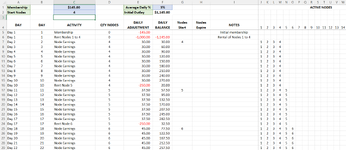
I have a spreadsheet that populates the data grid based on certain other calculations (which is all working fine) and I want to add a lookup function so that the data is only shown if the first entry in that column was less than 60 days ago. The challenge is that the spreadsheet does not have dates, it has days. Each event is a separate line, so there may be three or four events on any given day. The day number is in column A as "Day 1", "Day 2", etc and the number is extraced into hidden column B with the formula =RIGHT(A7,LEN(A7)-4).

The formula used to determine whether to enter data into a target column is =IF($B6-$B$5>59,"",IF(AND(MAX($G$5:$G7)>=J$4,J$4<=MAX($G$5:$G7)),J$4,"")). Column 1 data starts at row 7 in column J, column 2 data in column K may start on row 7 or below row 7. Column data 3 in column L may start at row 7 or below row 7. Each subsequent data column may start on the same row as it's predecessor, but never before it. Once populated, the data span should cover 60 days (which is what the IF($B6-$B$5>59 bit is trying to address. However, this only works correctly in data column 1 (J) because the start row of that data column is known to be day 1. However, for all subsequent data columns, I need to find the start day/row number of the first data point in that column and make reference to it in place of the $B$5 cell reference. I have tried VLOOKUP, HLOOKUP, LOOKUP, MATCH, INDIRECT and ROW in several combinations but must now confess to being massively confused about how to do this. Can anyone help?

 

[AndyGalloway]

For clarification, we just need to identify the row in which the formula starts returning a number rather than "". Then we need to identify the first row that appears 60 days later, so the value in column B would be that value + 59. The formula in all rows below that row should return "". The formula in all rows between the first row identified and the row 60 days late should return the number. It can't be that difficult, but I can't get my head around it.