Data Lookup

[IM_Haries]

Hello everyone


Let Me Introduce myself, i'm Harris and work on the university as academic administration.


i want to ask a question on here


Can excell looking Variable A and B in one row,


if met Variable A and B in the same row,
then retrieve the necessary data from the database sheet in the other sheet.


Can we create Excel formulas like that? I was very frustrated and confused.


i was looking for the formula on google but i was found nothing, then i found this forum,




I also provided screenshots for ease of friends in the forum to analyze the case.



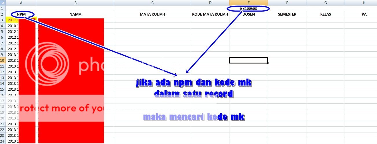
picture 1. the sheet where to put the formula.


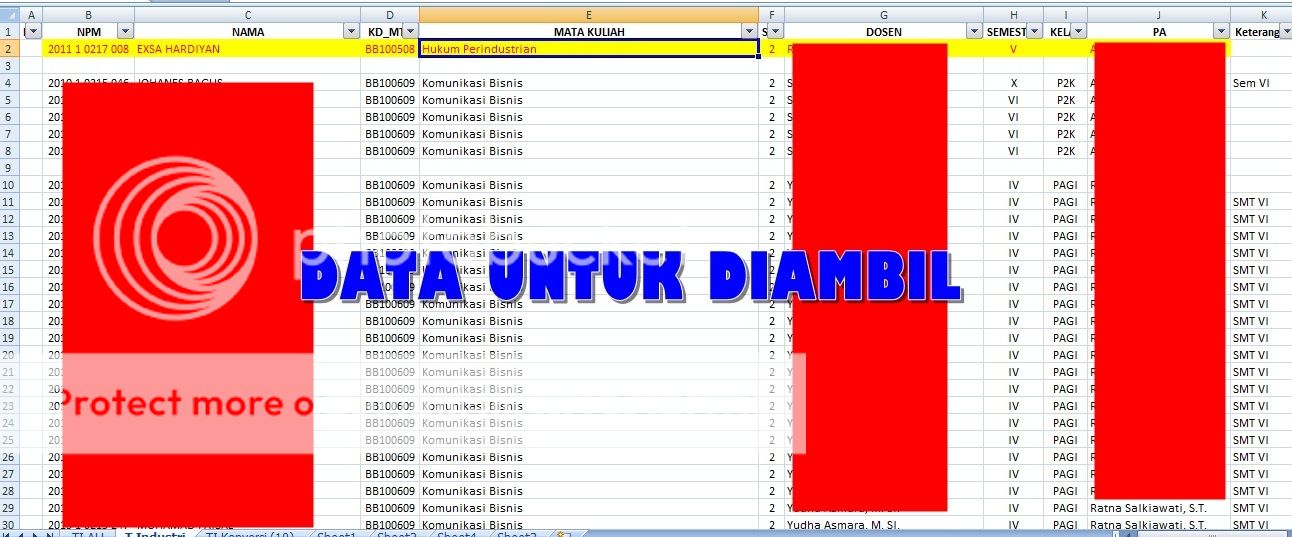
Picture. 2 it is the database sheet.



The formula that I need is, the formula to find "Kode_MK" and "NPM" (student identification number), and if successfully found the "NPM" and "MK code" of the same in a row, then search for "Mata_Kuliah" (Name of courses)


that is it, im sorry if my english so bad and will make you all confusing,

And Thank you for views and replies

 

[eliW]

Hi Haries, and welcome to the board!
It will be of help if you give a simple description of your data. E.g. column A -ID numbers, Column D - can contain same ID number, Column E -Course name etc. I want to match cells A and D on the same row. If it matches then....
It will help us to understand what you need
All the best,

 

[gaz_chops]

Hi Harris, it would be better if you could post a sample of your data instead of an image, see my signature for how to.

 

[IM_Haries]

Hi Haries, and welcome to the board!
It will be of help if you give a simple description of your data. E.g. column A -ID numbers, Column D - can contain same ID number, Column E -Course name etc. I want to match cells A and D on the same row. If it matches then....
It will help us to understand what you need
All the best,

Hi Harris, it would be better if you could post a sample of your data instead of an image, see my signature for how to.

Thanks EliW & gaz_chops ,

im so sorry if my data is so confusing (because the sheet & my language off course )
i will make this more simple to understand later, but in this time, im so confusing to finishing other deadline,

when im home, i will do this ASAP thx everyone

 

[IM_Haries]

Excel 2007

	A	B	C	D	E	F	G	H
1			BB100508
2	NPM	NAMA	MATA KULIAH	KODE MATA KULIAH	DOSEN	SEMESTER	KELAS	PA
3	2011 1 0217 008	a
4	2010 1 0215 046	b
5	2012 1 0215 210	c
6	2012 1 0215 323	d
7	2012 1 0215 324	e
8	2012 1 0215 326	f

<tbody>
</tbody>

final_sheet


​

Excel 2007

	B	C	D	E	F	G	H	I	J	K
1	NPM	NAMA	KD_MTK	MATA KULIAH	SKS	DOSEN	SEMESTER	KELAS	PA	Keterangan
2	2011 1 0217 008	a	BB100508	Hukum Perindustrian	2	xxx	V		xxx
3	2010 1 0215 046	b	BB100609	Komunikasi Bisnis	2	xxx.	X	P2K	xxx	Sem VI
4	2012 1 0215 210	c	BB100609	Komunikasi Bisnis	2	xxx.	VI	P2K	xxx
5	2012 1 0215 323	d	BB100609	Komunikasi Bisnis	2	xxx	VI	P2K	xxx
6	2012 1 0215 324	e	BB100609	Komunikasi Bisnis	2	xxx.	VI	P2K	xxx
7	2012 1 0215 326	f	BB100609	Komunikasi Bisnis	2	xxx	VI	P2K	xxx

<tbody>
</tbody>

db-sheet


​

Here it is,

it is simple (but make me confused )

i just want to fill the blank, and the data is from db-sheet

the logic is.... if found C2 (final sheet) and A3 (final sheet) on db_sheet, so finding A3 in db-sheet in the coloumn E,


i've tried to created the formula by myself, but im not so smart to found it,
Please everybody help me.

 

[MARK858]

Make sure the sheet name is exactly correct and most importantly you enter the formula without the curly brackets and then commit the formula with Ctrl Shift + Enter and not just Enter. If done correctly Excel will add the curly brackets. Do not try entering them manually.

Excel Workbook
	A	B	C	D	E	F	G	H
2	NPM	NAMA	MATA KULIAH	KODE MATA KULIAH	DOSEN	SEMESTER	KELAS	PA
3	2011 1 0217 008	a	Hukum Perindustrian
final_sheet

 

[MARK858]

Just filled out some other columns (The ones I could see you need). Instructions the same as in the last post (see quote)

Make sure the sheet name is exactly correct and most importantly you enter the formula without the curly brackets and then commit the formula with Ctrl Shift + Enter and not just Enter. If done correctly Excel will add the curly brackets. Do not try entering them manually.

Excel Workbook
	A	B	C	D	E	F	G	H
1			BB100508
2	NPM	NAMA	MATA KULIAH	KODE MATA KULIAH	DOSEN	SEMESTER	KELAS	PA
3	2011 1 0217 008	a	Hukum Perindustrian		xxx	V	0	xxx
final_sheet

 

[IM_Haries]

Just filled out some other columns (The ones I could see you need). Instructions the same as in the last post (see quote)


final_sheet

*	A	B	C	D	E	F	G	H
1	*	*	BB100508	*	*	*	*	*
2	NPM	NAMA	MATA KULIAH	KODE MATA KULIAH	DOSEN	SEMESTER	KELAS	PA
3	2011 1 0217 008	a	Hukum Perindustrian	*	xxx	V	0	xxx

<tbody>
</tbody>

Spreadsheet Formulas

Cell Formula C3 {=INDEX('db-sheet'!E:E,MATCH(1,(A3='db-sheet'!$B:$B)*(C1='db-sheet'!$D:$D),0))} E3 {=INDEX('db-sheet'!G:G,MATCH(1,(A3='db-sheet'!$B:$B)*(C1='db-sheet'!$D:$D),0))} F3 {=INDEX('db-sheet'!H:H,MATCH(1,(A3='db-sheet'!$B:$B)*(C1='db-sheet'!$D:$D),0))} G3 {=INDEX('db-sheet'!I:I,MATCH(1,(A3='db-sheet'!$B:$B)*(C1='db-sheet'!$D:$D),0))} H3 {=INDEX('db-sheet'!J:J,MATCH(1,(A3='db-sheet'!$B:$B)*(C1='db-sheet'!$D:$D),0))} <tbody> </tbody>

Formula Array: Produce enclosing { } by entering formula with CTRL+SHIFT+ENTER!

<tbody>
</tbody>

Excel tables to the web >> Excel Jeanie HTML 4

OH MY GOD...!!!

You Solving my case....

thank you MARK858, You are smart guy...

but, could you explain to me the detail why or how these formula work?

i can copy and paste it, but i don't know how it work,

and, what the mean "Do not try entering them manually?

so i must create the formula that could entering automatically?

THANK YOU VERY MUCH BTW....!!!

 

[MARK858]

"Do not try entering them manually?

I mean the curly brackets

enter the formula without the curly brackets and then commit the formula with Ctrl Shift + Enter and not just Enter. If done correctly Excel will add the curly brackets.

{=INDEX('db-sheet'!E:E,MATCH(1,(A3='db-sheet'!$B:$B)*(C1='db-sheet'!$D:$D),0))}

broken down...

'db-sheet'!E:E

The column you want the result to come from.

MATCH(1

it is an array formula and returns 0's and 1's (False and Trues). This says look for the 1 (True).

A3='db-sheet'!$B:$B

matches A3 with Column B of db-sheet

C1='db-sheet'!$D:$D

matches D3 with Column D of db-sheet

),0

asks for the matches to be exact matches.

Basically

MATCH(1,(A3='db-sheet'!$B:$B)*(C1='db-sheet'!$D:$D),0)

evaluates to 2
Then Index finds and returns the value from that position in the column

INDEX('db-sheet'!E:E,2) = E2

i can copy and paste it....
i must create the formula that could entering automatically

Need to do something with C1 first. Is that cell always static?

 

[IM_Haries]

You are the smart guy Mark,, however you explain this detailed, i still not so understand,
but Thank you very much for your genious helpp, could i ask u some questions?

where you learn the excel formula? just google it or you have a book or course?

and, in these data, actually i must solving the data ( a thousand row maybe) could you make this more automatically? if yes i will give you the data more detailed...

and... i have a gift for you (not money)