Data Validation Issue using List Option and Index/Match Formula

[CAROM16]

I have named ranges used in data validation to list corresponding information which the user can select from based on the PREVIOUS FIELD input. Consequently, I used index/match and vlookup functions to assess the previous input field and then display the correct corresponding list. HOWEVER, instead of displaying the list, it displays the NAME of the associated named range only! If I use the named range by itself (=named_range) it works fine and the correct data list is displayed. When I use the formula with either index/match or vlookup which (computes to "=named_range"), then the list shows "named_range" as the only option. I can use nested if functions which appear to work but it's crazy to have to do it that way (there are 20 options). In essence, I want Excel to recognize the computed "=named_range" for what it is - a defined list of data as opposed to recognizing it as a text field called "named_range"

I hope this isn't too nebulous. Please advise if I need to clarify with specific examples. Thank you for any light you can shine on this dilemma.

Regards - Dominick

 

[bobsan42]

Can you post some sample data and your validation range formula?
Have you tried including the check in the named range definition?
I don't have an answer for you now, but will try to play with it tomorrow.

 

[CAROM16]

Can you post some sample data and your validation range formula?
Have you tried including the check in the named range definition?
I don't have an answer for you now, but will try to play with it tomorrow.

Thank you so much for your response. I created a simple Xcel spread sheet which includes formulas and clearly shows the issue. However, I don't see a way to attach it - just images and the upload mini-sheet option (which I don't fully understand). Can you advise on the best way to transfer the Xcel file . Thank you

 

[bobsan42]

Upload it online (e.g. Google drive or OneDrive), share it and post the link.

 

[CAROM16]

Upload it online (e.g. Google drive or OneDrive), share it and post the link.

I copied the file to my Documents folder in One Drive as you suggested. Clicked on "Share" and it wanted to know who I want to share it with - displaying my contacts. Who do I click on and how do you get to read it? BTW, this is not my project, rather a very small and lucid explanation of the issue at hand. Once again, thank you for your time. (Never used One Drive before).

 

[bobsan42]

I copied the file to my Documents folder in One Drive as you suggested. Clicked on "Share" and it wanted to know who I want to share it with - displaying my contacts. Who do I click on and how do you get to read it? BTW, this is not my project, rather a very small and lucid explanation of the issue at hand. Once again, thank you for your time. (Never used One Drive before).

Select the link option. In this way you don't have to specify people, just send the link to anyone you like.

 

[bobsan42]

BTW. I came up with a working solution. Unfortunately I am using Office365.
At present I cannot build and test a solution for 2010.
I will post it here just for completeness. All the better if it works for you, but I suspect you may face some issues.

MrExcel Playbook 02 2021-09.xlsm
	A	B	C	D	E	F	G	H	I	J	K	L
1									VALS
2		LIST		VALS			LIST 1		a	b	c	d
3		a		a4			a		a1	b1	c1	d1
4							b		a2	b2	c2	d2
5							c		a3	b3	c3	d3
6		d		d2			d		a4	b4	c4	d4
7									a5	b5	c5	d5
8
9
10
11									VALS		Not Defined
12		a		a13					a	b
13									a11	b11
14		b		b12					a12	b12
15									a13
16		c		Not Defined					a14
17									a15
CAROM16

Cells with Data Validation
Cell	Allow	Criteria
B3	List	=$G$3:$G$6
B6	List	=$G$3:$G$6
B12	List	=$G$3:$G$6
B14	List	=$G$3:$G$6
B16	List	=$G$3:$G$6
D3	List	=OFFSET($I$2,1,MATCH($B3,$I$2#,0)-1,5,1)
D6	List	=OFFSET($I$2,1,MATCH($B6,$I$2#,0)-1,5,1)
D12	List	=IF($B12="a",Aval,IF($B12="b",Bval,$K$11))
D14	List	=IF($B14="a",Aval,IF($B14="b",Bval,$K$11))
D16	List	=IF($B16="a",Aval,IF($B16="b",Bval,$K$11))

I have selected a LIST as a validation Allow option. This allows to have an in-cell dropdown.
The validation formulas self-adjust when you copy paste the pair of cells in columns B & D
The yellow and orrange ranges are solution version 1.
The greens are version 2 - with Named Ranges.
I don't know why it is not shown here but there are two named ranges:
Aval - i13:i17
Bval - J13:J14

 

[CAROM16]

Thank you for your time, patience, and effort - especially in light of no one else took the time to respond. Unfortunately, it appears I was unable to effectively communicate my issue/concerns regarding formulas (specifically named ranges utilizing Index/Match and Vlookup) in the list option of Data Validations. I wish you the best of luck in your endeavors.

 

[Akuini]

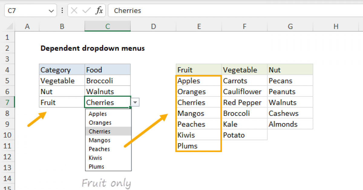
It looks like what you want is dependent data validation.
Try using Indirect function, like this:

How to make dependent dropdown lists in Excel

One of the most useful features of data validation is the ability to create a dropdown list that let users select a value from a predefined list. But how can you make one dropdown dynamically respond to another? In other words, how can you make the values in a dropdown list depend on another...

exceljet.net

 

[bobsan42]

Certainty the mini-sheet in post #7 i about dependent data validation. The validation of the colored cells in column D changes according to the values of the cells in column B.