Data Validation list to have a certain value

[craigwojo]

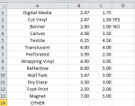
In a Data Validation cell, I need to have a value for each item. If they pick "Digital Media" in E3 then the value would be 1.50. The items associated with the cell are (=Sheet2!A1:A14).
How is this done?

 

[jasonb75]

It needs a change to the existing formulas in N3 and P3 which is why I asked what those formulas are.

 

[craigwojo]

Is there a way I could send you my spreadsheet?

 

[jasonb75]

I don't see that it would be necessary, you only need to copy the formulas from the cells, but if you need to, you can post sections of your sheet using XL2BB

XL2BB - Excel Range to BBCode

Excel 'mini-sheet' in messages - XL2BB Although experts prefer to read your description and question instead of working in your actual file to solve your problem, there are times that it is difficult to explain an issue without providing actual...

www.mrexcel.com

 

[craigwojo]

I'm sorry. I added another column in the spreadsheet and it shifted some columns.

In K3 I need to add .20 per sqft if "YES' in cell "L3" is chose (=Sheet2!$D$1:$D$3) the cell that contains "YES" is D2.

Also, if M3 is "YES" it will add 10% to O3 (=VLOOKUP(E3,Sheet2!$A$1:$B$14,2,0) and Q3 (=VLOOKUP(E3,Sheet2!$A$1:$C$14,3,0).

Also, I attached Sheet 2 that has all the data lists for Data Validation and VLOOKUP.

Again, Thank you so much.

God bless,
Craig

 

[jasonb75]

This should do it, new formula for O3 =VLOOKUP(E3,Sheet2!$A$1:$B$14,2,0)+IF(L3="YES",0.20,0)

For Q3 =VLOOKUP(E3,Sheet2!$A$1:$C$14,3,0)*IF(M3="YES",1.1,1)

 

[craigwojo]

This should do it, new formula for O3 =VLOOKUP(E3,Sheet2!$A$1:$B$14,2,0)+IF(L3="YES",0.20,0)

For Q3 =VLOOKUP(E3,Sheet2!$A$1:$C$14,3,0)*IF(M3="YES",1.1,1)

OK. I'm sorry if I messed up but, M3 would increase both O3 and Q3 10%.

While L3 would only effect Q3 adding 0.20 per sqft in J3.

Thank you.

 

[jasonb75]

If L3 and M3 are both "YES" which should be added to Q3 first, $0.20 or 10%?

Starting with $1.00 in Q3, should the result be $1.32 ($0.20 added before 10%) or $1.30 ($0.20 added after 10%)?

 

[craigwojo]

If L3 and M3 are both "YES" which should be added to Q3 first, $0.20, or 10%?

Starting with $1.00 in Q3, should the result be $1.32 ($0.20 added before 10%) or $1.30 ($0.20 added after 10%)?

First, add the 10% then 0.20 would be added after.
$1.30 ($0.20 added after 10%)

I hope this is what you're asking.

 

[jasonb75]

I think this should do it (not tested)

=VLOOKUP(E3,Sheet2!$A$1:$B$14,2,0)*IF(M3="YES",1.1,1)+IF(L3="YES",0.20,0)

 

[craigwojo]

Thank you for everything. I did a little tweaking and learned some.

Thank you and God bless,
Craig