Date from row of dates corresponding to first non-blank cell in other row

[salange]

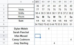
Hi all - this spreadsheet is for tracking volunteers at a wildlife center. I need a formula that returns the first date that a volunteer showed up this year. Each cell from BN7 down and right contains the number of hours that each vol worked on each day. So basically, for each vol, I need a formula that returns the date in row 5 that corresponds with the first non-blank cell for that vol past BN. Dylan should return 1/3, Sarah and Irfan should return a blank or an error or whatever, Casey should return 1/7, etc.

I think it should involve an array formula and maybe SORT but past that I'm pretty stumped. Any help would be much appreciated - thanks!

(I'm actually using Google Sheets but didn't get any bites in that forum so I'll take an Excel solution and translate it myself. Thanks!)

 

[James006]

Hi,
Not sure to fully understand your question ...
But, usually, to get the value of your first non-blank cell in a given range, you could use the following Array formula:

=INDEX(yourRange,MATCH(FALSE,ISBLANK(yourRange),0))}

 

[salange]

Thank you for the response! That formula works as you said, but I don't ultimately want the value of the first non-blank cell. I want the date that the first non-blank cell corresponds with. In the image attached above, you can see the dates in row 5 and the names in rows 7, 8, 9, etc. So for Dylan, your formula returns "4," which is indeed the number of hours he worked on his first day, but I want it to return "1/3" to tell me he worked those hours on January 3.

Any additional help would be most appreciated! Thank you!

 

[salange]

I made a mini-sheet in Excel to hopefully communicate more clearly what I'm looking for. In this version, the formula I want goes in column B, and it should return 1/2/23 for Alice, 1/3/23 for Bob, and 1/1/23 for Carrie. Thank you in advance for any help y'all can provide!

scott's test file.xlsx
	A	B	C	D	E	F	G
1	Name	First Date Worked	1/1/2023	1/2/2023	1/3/2023	1/4/2023	1/5/2023
2	Alice			3		4
3	Bob				4		2
4	Carrie		8				5
Sheet1

 

[salange]

I figured it out - just a minor adjustment to James006's formula. The first "YourRange" should be the date range and the second one should be volunteer's hour range. So in my original spreadsheet, it's:

={(INDEX(BN$5:PN$5,MATCH(FALSE,ISBLANK(BN7:PN7),0))}

Thanks!

 

[James006]

OK ...
There is just a minor adjustement to be made...
Index should refer to row 1 ... and your match to the rows you need to analyze ...

 

[salange]

Thanks, James!

 

[James006]

Glad you managed to fix your problem

 

[Peter_SSs]

You would have to adjust the ranges but what about just this?

23 03 01.xlsm
	B	C	D	E	F	G
1	First Date Worked	1/01/2023	1/02/2023	1/03/2023	1/04/2023	1/05/2023
2	1/02/2023		3		4
3	1/03/2023			4		2
4	1/01/2023	8				5
First Date

Cell Formulas
Range	Formula
B2:B4	B2	=MINIFS(C$1:G$1,C2:G2,"<>")