Dates Help! Using SUMPRODUCT,MONTH<ROW< INDIRECT and network days

sgibbs183

New Member
Joined
Aug 5, 2020
Messages
28
Office Version
  1. 365
  2. 2013
Platform
  1. Windows
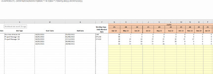
I have a sheet below where I need to calculate how many days between the start and end date fall into that period. I have done this, so for example, 30 days falls into April from start date 28/03/2022 to end date 01/05/2022. But I want to know how many of these days are NETWORKDAYS so I can times this amount by the blended rate.

Is there anyone that can help please!

1674123140626.png
 

Attachments

  • 1674123018850.png
    1674123018850.png
    28 KB · Views: 5
In that case can post some sample data.

MrExcel has a tool called “XL2BB” that lets you post samples of your data that will allow us to copy/paste it to our Excel spreadsheets, so we can work with the same copy of data that you are. Instructions on using this tool can be found here: XL2BB Add-in

Note that there is also a "Test Here” forum on this board. This is a place where you can test using this tool (or any other posting techniques that you want to test) before trying to use those tools in your actual posts.
 
Upvote 0

Excel Facts

Format cells as date
Select range and press Ctrl+Shift+3 to format cells as date. (Shift 3 is the # sign which sort of looks like a small calendar).
The following may help. You can review the formulas and then try the concepts on your sheet.
If you workdays are different, edit the formula for appropriate Workdays.
You can also refer to a list of holiday dates.

T202212a.xlsm
ABCDEFGHIJKLMNO
1Days /Workdays in period
21-Jan-221-Feb-221-Mar-221-Apr-221-May-221-Jun-221-Jul-221-Aug-221-Sep-221-Oct-221-Nov-221-Dec-22
3StartEnd
415-Dec-2115-Mar-22212011000000000
55-May-2215-Feb-2300001922212322212222
610-Jan-2220-Oct-221620232122222123221400
72-Feb-2226-Sep-2201923212222212318000
81-Jan-2231-Mar-22212023000000000
91-Jan-2231-Dec-22212023212222212322212222
2aa
Cell Formulas
RangeFormula
D4:O9D4=MAX(0,NETWORKDAYS.INTL(MAX($A4,D$2),MIN($B4,EOMONTH(D$2,0)),1))
 
Upvote 0
In that case can post some sample data.

MrExcel has a tool called “XL2BB” that lets you post samples of your data that will allow us to copy/paste it to our Excel spreadsheets, so we can work with the same copy of data that you are. Instructions on using this tool can be found here: XL2BB Add-in

Note that there is also a "Test Here” forum on this board. This is a place where you can test using this tool (or any other posting techniques that you want to test) before trying to use those tools in your actual posts.
Resource .xlsx
ABCDEFGHIJKLMNOPQR
122/23
2Working Days252020252020252020252020
3Period Start Date28/03/202202/05/202230/05/202227/06/202201/08/202229/08/202226/09/202231/10/202228/11/202226/12/202230/01/202327/02/2023
4InputSelectPeriod End Date01/05/202229/05/202226/06/202231/07/202228/08/202225/09/202230/10/202227/11/202225/12/202229/01/202326/02/202326/03/2023
5Line NumberDetailed descriptionJob TypeStart DateEnd DateDaily Blended RateApr 22May 22Jun 22Jul 22Aug 22Sep 22Oct 22Nov 22Dec 22Jan 23Feb 23Mar 23
61Business Analyst 3B28/03/202210/05/2023240252020252020252020252020
72Business Analyst 3B28/03/202201/05/202224025           
83Project Manager 3A28/03/202227/11/2022574.962520202520202520    
9420/04/202230/09/2022 820202520205     
10528/03/202228/08/2022 2520202520       
116            
127            
138            
2. Resource
Cell Formulas
RangeFormula
G2G2=NETWORKDAYS(INDEX('[BCM _ SG NEW.xlsx]Validation'!$AD$2:$AD$73,MATCH('2. Resource'!G5,'[BCM _ SG NEW.xlsx]Validation'!$AC$2:$AC$73,0)),INDEX('[BCM _ SG NEW.xlsx]Validation'!$AE$2:$AE$73,MATCH('2. Resource'!G5,'[BCM _ SG NEW.xlsx]Validation'!$AC$2:$AC$73,0)))
H2:R2H2=NETWORKDAYS(INDEX('[BCM _ SG NEW.xlsx]Validation'!$AD$2:$AD$73,MATCH('2. Resource'!H5,'[BCM _ SG NEW.xlsx]Validation'!$AC$2:$AC$73,0)),INDEX('[BCM _ SG NEW.xlsx]Validation'!$AE$2:$AE$73,MATCH('2. Resource'!H5,'[BCM _ SG NEW.xlsx]Validation'!$AC$2:$AC$73,0)))
G3:R3G3=INDEX('[BCM _ SG NEW.xlsx]Validation'!$AD$2:$AD$73,MATCH(G5,'[BCM _ SG NEW.xlsx]Validation'!$AC$2:$AC$73,0))
G4:R4G4=INDEX('[BCM _ SG NEW.xlsx]Validation'!$AE$2:$AE$73,MATCH(G5,'[BCM _ SG NEW.xlsx]Validation'!$AC$2:$AC$73,0))
G6:R10H6=IF(NETWORKDAYS(MAX($D6,H$3),MIN($E6,H$4))>1,NETWORKDAYS(MAX($D6,H$3),MIN($E6,H$4)),"")
H11:R13H11=IFERROR(H$2*$F11,"")
F6:F13F6=IFERROR(VLOOKUP(C6,'[BCM _ SG NEW.xlsx]Validation'!V:X,3,0),"")
Press CTRL+SHIFT+ENTER to enter array formulas.
Cells with Conditional Formatting
CellConditionCell FormatStop If True
H13:BZ62Cell Value=0textNO
H11:BZ11Cell Value=0textNO
H12:BZ12Cell Value=0textNO
 
Upvote 0
Resource .xlsx
ABCDEFGHIJKLMNOPQR
122/23
2Working Days252020252020252020252020
3Period Start Date28/03/202202/05/202230/05/202227/06/202201/08/202229/08/202226/09/202231/10/202228/11/202226/12/202230/01/202327/02/2023
4InputSelectPeriod End Date01/05/202229/05/202226/06/202231/07/202228/08/202225/09/202230/10/202227/11/202225/12/202229/01/202326/02/202326/03/2023
5Line NumberDetailed descriptionJob TypeStart DateEnd DateDaily Blended RateApr 22May 22Jun 22Jul 22Aug 22Sep 22Oct 22Nov 22Dec 22Jan 23Feb 23Mar 23
61Business Analyst 3B28/03/202210/05/2023240252020252020252020252020
72Business Analyst 3B28/03/202201/05/202224025           
83Project Manager 3A28/03/202227/11/2022574.962520202520202520    
9420/04/202230/09/2022 820202520205     
10528/03/202228/08/2022 2520202520       
116            
127            
138            
2. Resource
Cell Formulas
RangeFormula
G2G2=NETWORKDAYS(INDEX('[BCM _ SG NEW.xlsx]Validation'!$AD$2:$AD$73,MATCH('2. Resource'!G5,'[BCM _ SG NEW.xlsx]Validation'!$AC$2:$AC$73,0)),INDEX('[BCM _ SG NEW.xlsx]Validation'!$AE$2:$AE$73,MATCH('2. Resource'!G5,'[BCM _ SG NEW.xlsx]Validation'!$AC$2:$AC$73,0)))
H2:R2H2=NETWORKDAYS(INDEX('[BCM _ SG NEW.xlsx]Validation'!$AD$2:$AD$73,MATCH('2. Resource'!H5,'[BCM _ SG NEW.xlsx]Validation'!$AC$2:$AC$73,0)),INDEX('[BCM _ SG NEW.xlsx]Validation'!$AE$2:$AE$73,MATCH('2. Resource'!H5,'[BCM _ SG NEW.xlsx]Validation'!$AC$2:$AC$73,0)))
G3:R3G3=INDEX('[BCM _ SG NEW.xlsx]Validation'!$AD$2:$AD$73,MATCH(G5,'[BCM _ SG NEW.xlsx]Validation'!$AC$2:$AC$73,0))
G4:R4G4=INDEX('[BCM _ SG NEW.xlsx]Validation'!$AE$2:$AE$73,MATCH(G5,'[BCM _ SG NEW.xlsx]Validation'!$AC$2:$AC$73,0))
G6:R10H6=IF(NETWORKDAYS(MAX($D6,H$3),MIN($E6,H$4))>1,NETWORKDAYS(MAX($D6,H$3),MIN($E6,H$4)),"")
H11:R13H11=IFERROR(H$2*$F11,"")
F6:F13F6=IFERROR(VLOOKUP(C6,'[BCM _ SG NEW.xlsx]Validation'!V:X,3,0),"")
Press CTRL+SHIFT+ENTER to enter array formulas.
Cells with Conditional Formatting
CellConditionCell FormatStop If True
H13:BZ62Cell Value=0textNO
H11:BZ11Cell Value=0textNO
H12:BZ12Cell Value=0textNO
This seems to work thank you so much!! :)
 
Upvote 0
You're welcome & thanks for the feedback.
 
Upvote 0

Forum statistics

Threads
1,214,651
Messages
6,120,744
Members
448,989
Latest member
mariah3

We've detected that you are using an adblocker.

We have a great community of people providing Excel help here, but the hosting costs are enormous. You can help keep this site running by allowing ads on MrExcel.com.
Allow Ads at MrExcel

Which adblocker are you using?

Disable AdBlock

Follow these easy steps to disable AdBlock

1)Click on the icon in the browser’s toolbar.
2)Click on the icon in the browser’s toolbar.
2)Click on the "Pause on this site" option.
Go back

Disable AdBlock Plus

Follow these easy steps to disable AdBlock Plus

1)Click on the icon in the browser’s toolbar.
2)Click on the toggle to disable it for "mrexcel.com".
Go back

Disable uBlock Origin

Follow these easy steps to disable uBlock Origin

1)Click on the icon in the browser’s toolbar.
2)Click on the "Power" button.
3)Click on the "Refresh" button.
Go back

Disable uBlock

Follow these easy steps to disable uBlock

1)Click on the icon in the browser’s toolbar.
2)Click on the "Power" button.
3)Click on the "Refresh" button.
Go back
Back
Top