Dealing with a Matrix of Data using Offset Beginning Rows

[EVANWIT84]

Hi All,

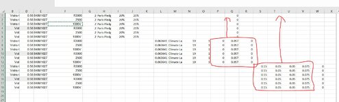
I'm dealing with a matrix of data where I have accounts off to the far left and the data repeats and where there are empty cells I just want to shift the data up. My problem is that in Range P thru R can be blank and S thru V can also be blank at the same time. As a result, I receive a Run-Time Error 1004 since the copy/paste are not the same size. I have also stuggled to write an If Statement that would solve this so i'm back to the drawing board.

Lastly, once I have shifted all the data up then I will delete out un-needed rows and copy/paste into a new tab. This part I should be able to do on my own.

Sub GrabDataForEachAccount()
Dim x As Range
Dim xRange As Range
Dim amf As Worksheet
Dim ws As Worksheet
Dim rd As Worksheet
Dim Cal As Worksheet
Dim rdLastCell As Long
Dim FirstRow As Double
Dim LastRow As Double


Set ws = Sheets("Summary")
Set amf = Sheets("AMF")
Set Cal = Sheets("CalcSheet")

Set xRange = amf.Range("a2:a" & amf.Range("a1048567").End(xlUp).Row)


FirstRow = Cal.Range("P1", "P" & Rows.Count).End(xlDown).Row
LastRow = Cal.Range("P" & Rows.Count).End(xlUp).Row

Application.ScreenUpdating = False

For Each x In xRange.Cells

ws.UsedRange.SpecialCells(xlCellTypeVisible).AutoFilter Field:=5, Criteria1:=x
ws.UsedRange.SpecialCells(xlCellTypeVisible).Copy Sheets("CalcSheet").[a1]
Cal.Range("P" & FirstRow, "R" & LastRow).Copy Cal.Range("P2") 'I want this to Copy if >0 Values in Range
Cal.Range("AB" & FirstRow, "AB" & LastRow).Copy Cal.Range("AB2")

Cal.UsedRange.SpecialCells(xlCellTypeVisible).AutoFilter Field:=9, Criteria1:=">0"
Cal.UsedRange.SpecialCells(xlCellTypeVisible).Copy Sheets("Summary2").[a1]

'Delete unneeded rows
'Paste into new tab and add into bottom

Cal.Cells.Clear

Next

End Sub

 

[aRandomHelper]

I have accounts off to the far left and the data repeats

Is it always the same number of rows if/when data appears in, say, column G or H?

Meaning, if I see 10 rows of data on column G/H, would I see also 10 rows of data for the P-R chunk, and also 10 rows for S-V chunk?

If the answer is yes, then you might be able to work around this idea.

 

[EVANWIT84]

Well the rows would be the same but based on the ratings it could be 5 rows repeating or 10 rows repeating. The repeating pattern is the same but the variable can change if that makes sense?

 

[aRandomHelper]

So, get the last row based on column G/H.
If there's a header row, using this last row - 1 will give the number of rows that it repeats. If there's no header row, then the last row would be the number of rows.

Based on this number, to grab the corresponding number of rows starting from last row+1, column P, resize the range to Number of rows = last row, Number of columns = 3.

Next, go to last row+last row+1, and grab from column S. Likewise, resize the range to Number of rows = last row, Number of columns = 4.

I am not on my computer now so I can't provide a code. If you still have trouble making it work, I'll come up with something tomorrow.

 

[EVANWIT84]

Thanks, let me look and see if I can apply it. I also think the problem though is that this won't account for when P is empty unless i'm missing something.

 

[EVANWIT84]

I think I got it...made a few tweaks as I don't completely understand the resize. I'm now going to delete the columns I don't need and just condense to what's essential. This script gets me what I need unless there's a better way to eliminate the offset and only use the resize?

Dim xRange As Range

Dim Cal As Worksheet

Dim FirstRow As Double
Dim LastRow As Double
Dim LastRowI As Double


Set Cal = Sheets("CalcSheet")

FirstRow = Cal.Range("l1", "l" & Rows.Count).End(xlDown).Row
LastRow = Cal.Range("h" & Rows.Count).End(xlUp).Row
LastRowI = Cal.Range("I" & Rows.Count).End(xlUp).Row

Range("H" & LastRow + 1).Offset(0, 1).Resize(LastRow, 2).Copy Cal.Range("i2")

 

[aRandomHelper]

Good that you got something going!

I'm now going to delete the columns I don't need and just condense to what's essential

So what are the columns remaining now? I see you're now getting the last row based on column H, and you're copying that to column I? I thought column H contains the first "set" of data that would be at the top?

Anyway, let me explain what I meant on my last post with a picture, might be easier to understand.

So with reference to my screenshot as the data set, the code would look something like this:

Sub abc()
    Dim Cal As Worksheet
   
    Dim FirstRow As Long
    Dim LastRow As Long
   
    Set Cal = Sheets("CalcSheet")
   
    'LastRow = Cal.Range("h" & Rows.Count).End(xlUp).Row
    LastRow = Cal.Cells(Rows.Count, "H").End(xlUp).Row 'You can also use Cells instead of Range
       
    Cal.Cells(LastRow + 1, "K").Resize(LastRow, 3).Copy Cal.Cells(1, "K")
    Cal.Cells(LastRow + LastRow + 1, "N").Resize(LastRow, 4).Copy Cal.Cells(1, "N")
End Sub