Deduplicate data depending on various date conditions

mayasak

New Member
Joined
Jan 30, 2022
Messages
2
Office Version
  1. 365
Platform
  1. Windows
Hi,

I have a data set with patient duplicates. I need to remove duplicates depending on certain dates and conditions (events).
For "disease" = Auris, keep only the first observation if "id" and "DOB" are identical. Remove all other observations.
For "disease" = Acino, keep only first and last obs if "id" and "DOB" are identical.
For "disease" = CRE, if "id" and "DOB" are identical, keep the first observation and next observation(s) if they have a date difference of more than 12 months from the previous observation. Else keep the first obs and delete the observations with a < 12 months date difference.
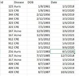
I've uploaded a mini-sheet that has the original data and an image for the resulted deduplicated data.
Please advise.
testdedup (3).xlsx
ABCD
1IdDiseaseDOBDate
2123Auris1/8/19611/1/2018
3123CRE1/8/19619/2/2020
4344CRE2/12/19568/6/2019
5344CRE2/12/19563/6/2020
6344CRE2/12/19563/3/2022
7323CRE7/1/19931/6/2019
8323CRE7/1/19939/6/2020
9323CRE7/1/19939/30/2020
10167Acino12/9/20013/6/2019
11167Acino12/9/20014/30/2020
12167Acino12/9/20019/3/2021
13912CRE3/1/20123/3/2018
14912CRE3/1/20125/6/2019
15912CRE3/1/20129/6/2020
16256Auris5/27/19838/5/2020
17256Auris5/27/198312/7/2020
18256Auris5/27/198310/7/2021
19256Auris5/27/19832/7/2022
20317Acino7/17/198512/7/2018
21317Acino7/17/19851/3/2018
22409CRE8/7/19873/3/2018
23409CRE8/7/19875/6/2019
24409CRE8/7/19879/6/2019
25409CRE8/7/198710/6/2021
Testdedup
 

Attachments

  • deduplcated data.JPG
    deduplcated data.JPG
    84.9 KB · Views: 12

Excel Facts

Save Often
If you start asking yourself if now is a good time to save your Excel workbook, the answer is Yes
This is a tricky problem and I'm not aware of a way to do it without some helper columns, although someone might have a clever solution. Because there are different criteria for filtering each of the disease names, and some of those criteria involve determining whether any observation dates come after or before the date on any given row, I resorted to a solution that looks up the table and down the table. To make this work, the initial data set is re-created, but sorted in a specific order using this formula:
Excel Formula:
=SORT($A$2:$D$25,{1,2,4})
This will result in the entire data table "spilling" across columns and down rows in a certain order. This assumes the original source table is in the range $A$2:$D$25 and in column order shown in the example {Id, Disease, DOB, Date}. In this example, the SORT formula above is entered into cell F2, and after "spilling", columns F:I contain the sorted table. Then logic/filtering rules are applied to that sorted table. The logic/filtering rules are given in this formula:
Excel Formula:
=LET(rcnt, COUNTA(INDEX($F$2#,,1)),
          idx,   SUM(IF(OR($G2="Auris",$G2="Acino",$G2="CRE"),IF(COUNTIFS($F$2:$F2,$F2,$G$2:$G2,$G2,$H$2:$H2,$H2)=1,ROWS($G$2:$G2),0),0),
                     IF($G2="Acino",IF(COUNTIFS($F2:INDEX($F$2#,rcnt,1),$F2,$G2:INDEX($F$2#,rcnt,2),$G2,$H2:INDEX($F$2#,rcnt,3),$H2)=1,ROWS($G$2:$G2),0),0),
                     IF($G2="CRE",IF(EDATE($I2,-12)>=XLOOKUP(1,(($F1:$F$2=$F2)*($G1:$G$2=$G2)*($H1:$H$2=$H2)*($J1:$J$2>0)),$I1:$I$2,"",0,-1),ROWS($I$2:$I2),0),0)),
          idx)
The 1st component of the LET function is a formula to determine how many rows are in the sorted table...the row count, or rcnt. The 2nd component determines the row index if that particular row in the sorted table should be included in final result. If not, then a 0 is returned. This index-determining step occurs in a formula called idx, and it consists of three parts, each beginning with an IF statement inside the SUM function. The first of those finds the first occasion (based on date) for every unique combination of Id/Disease/DOB in the sorted table. The second of those finds the last occasion (based on date) for every combination of Id/Disease/DOB where the Disease="Acino" in the sorted table. The third of those looks up the helper column to find the most recent occasion (based on date) that has already been identified for inclusion in the results table for every combination of Id/Disease/DOB where the Disease="CRE". That date is compared with the current row's observation Date, and if the difference is >= 1 yr, then the current row's index is also included in the helper column. Because each of these three parts of the idx formula are mutually exclusive, the values resulting from each part can be summed to create a single helper column containing either the row index of interest or 0's. In practice, the helper column formula is pasted beside the sorted table and copied down to match the entire length of the sorted table. In this example, the helper column formula is pasted into J2 and pulled down.
Finally, the results table is generated with this formula:
Excel Formula:
=LET(rcnt,COUNTA(INDEX($F$2#,,1)), idx,OFFSET($J$2,,,rcnt,1), fidx,FILTER(idx,idx<>0),INDEX($F$2#,fidx,{1,2,3,4}))
You will see that this formula references the upper left cell of the sorted table ($F$2#) and the top of the helper column ($J$2).
MrExcel_20220529_v2.xlsx
ABCDEFGHIJKLMNO
1IdDiseaseDOBDateIdDiseaseDOBDateRules HelperIdDiseaseDOBDate
2123Auris1/8/19611/1/2018123Auris1/8/19611/1/20181123Auris1/8/19611/1/2018
3123CRE1/8/19619/2/2020123CRE1/8/19619/2/20202123CRE1/8/19619/2/2020
4344CRE2/12/19568/6/2019167Acino12/9/20013/6/20193167Acino12/9/20013/6/2019
5344CRE2/12/19563/6/2020167Acino12/9/20014/30/20200167Acino12/9/20019/3/2021
6344CRE2/12/19563/3/2022167Acino12/9/20019/3/20215256Auris5/27/19838/5/2020
7323CRE7/1/19931/6/2019256Auris5/27/19838/5/20206317Acino7/17/19851/3/2018
8323CRE7/1/19939/6/2020256Auris5/27/198312/7/20200317Acino7/17/198512/7/2018
9323CRE7/1/19939/30/2020256Auris5/27/198310/7/20210323CRE7/1/19931/6/2019
10167Acino12/9/20013/6/2019256Auris5/27/19832/7/20220323CRE7/1/19939/6/2020
11167Acino12/9/20014/30/2020317Acino7/17/19851/3/201810344CRE2/12/19568/6/2019
12167Acino12/9/20019/3/2021317Acino7/17/198512/7/201811344CRE2/12/19563/3/2022
13912CRE3/1/20123/3/2018323CRE7/1/19931/6/201912409CRE8/7/19873/3/2018
14912CRE3/1/20125/6/2019323CRE7/1/19939/6/202013409CRE8/7/19875/6/2019
15912CRE3/1/20129/6/2020323CRE7/1/19939/30/20200409CRE8/7/198710/6/2021
16256Auris5/27/19838/5/2020344CRE2/12/19568/6/201915912CRE3/1/20123/3/2018
17256Auris5/27/198312/7/2020344CRE2/12/19563/6/20200912CRE3/1/20125/6/2019
18256Auris5/27/198310/7/2021344CRE2/12/19563/3/202217912CRE3/1/20129/6/2020
19256Auris5/27/19832/7/2022409CRE8/7/19873/3/201818
20317Acino7/17/198512/7/2018409CRE8/7/19875/6/201919
21317Acino7/17/19851/3/2018409CRE8/7/19879/6/20190
22409CRE8/7/19873/3/2018409CRE8/7/198710/6/202121
23409CRE8/7/19875/6/2019912CRE3/1/20123/3/201822
24409CRE8/7/19879/6/2019912CRE3/1/20125/6/201923
25409CRE8/7/198710/6/2021912CRE3/1/20129/6/202024
Sheet3
Cell Formulas
RangeFormula
F2:I25F2=SORT($A$2:$D$25,{1,2,4})
L2:O18L2=LET(rcnt,COUNTA(INDEX($F$2#,,1)), idx,OFFSET($J$2,,,rcnt,1), fidx,FILTER(idx,idx<>0),INDEX($F$2#,fidx,{1,2,3,4}))
J2:J3J2=LET(rcnt, COUNTA(INDEX($F$2#,,1)), idx, SUM( IF(OR($G2="Auris",$G2="Acino",$G2="CRE"),IF(COUNTIFS($F$2:$F2,$F2,$G$2:$G2,$G2,$H$2:$H2,$H2)=1,ROWS($G$2:$G2),0),0), IF($G2="Acino",IF(COUNTIFS($F2:INDEX($F$2#,rcnt,1),$F2,$G2:INDEX($F$2#,rcnt,2),$G2,$H2:INDEX($F$2#,rcnt,3),$H2)=1,ROWS($G$2:$G2),0),0), IF($G2="CRE",IF(EDATE($I2,-12)>=XLOOKUP(1,(($F1:$F$2=$F2)*($G1:$G$2=$G2)*($H1:$H$2=$H2)*($J1:$J$2>0)),$I1:$I$2,"",0,-1),ROWS($I$2:$I2),0),0)), idx)
J4:J25J4=LET(rcnt, COUNTA(INDEX($F$2#,,1)), idx, SUM( IF(OR($G4="Auris",$G4="Acino",$G4="CRE"),IF(COUNTIFS($F$2:$F4,$F4,$G$2:$G4,$G4,$H$2:$H4,$H4)=1,ROWS($G$2:$G4),0),0), IF($G4="Acino",IF(COUNTIFS($F4:INDEX($F$2#,rcnt,1),$F4,$G4:INDEX($F$2#,rcnt,2),$G4,$H4:INDEX($F$2#,rcnt,3),$H4)=1,ROWS($G$2:$G4),0),0), IF($G4="CRE",IF(EDATE($I4,-12)>=XLOOKUP(1,(($F$2:$F3=$F4)*($G$2:$G3=$G4)*($H$2:$H3=$H4)*($J$2:$J3>0)),$I$2:$I3,"",0,-1),ROWS($I$2:$I4),0),0)), idx)
Dynamic array formulas.
 
Upvote 0
Here is a macro for you to consider.

The macro sorts the data in column A, B, C, and D. The results are put in cell F2 onwards.

VBA Code:
Sub remove_duplicates()
  Dim datos As Range
  Dim dic As Object
  Dim keep As Boolean
  Dim i As Long, j As Long, y As Long
  Dim dtbefore As Date, dtnew As Date
  Dim ky As Variant, a As Variant, b As Variant
  
  Set datos = Range("A1", Range("D" & Rows.Count).End(3))
  datos.Sort Key1:=Range("D1"), Order1:=xlAscending, Header:=xlYes
  datos.Sort Key1:=Range("A1"), Order1:=xlAscending, _
             Key2:=Range("B1"), Order2:=xlAscending, _
             Key3:=Range("C1"), Order3:=xlAscending, Header:=xlYes
  
  a = datos.Value
  ReDim b(1 To UBound(a, 1), 1 To UBound(a, 2))
  Set dic = CreateObject("Scripting.Dictionary")
  
  'remove duplicates depending on certain dates and conditions
  For i = 2 To UBound(a, 1)
    ky = a(i, 1) & "|" & a(i, 2)
    keep = False
    If Not dic.exists(ky) Then
      y = y + 1
      dic(ky) = y & "|" & 1 & "|" & a(i, 4)
      keep = True
    Else
      Select Case LCase(a(i, 2))
      Case LCase("Auris")         'keep only the first
      
      Case LCase("CRE")           'keep first and next if they have a date more than 12 months
        dtbefore = b(j, 4)
        dtnew = DateSerial(Year(dtbefore), Month(dtbefore) + 12, Day(dtbefore))
        If a(i, 4) > dtnew Then
          y = y + 1
          dic(ky) = y & "|" & 1 & "|" & a(i, 4)
          keep = True
        End If
        
      Case LCase("Acino")         'keep first and last
        If Split(dic(ky), "|")(1) = 1 Then y = y + 1
        dic(ky) = y & "|" & 2 & "|" & a(i, 4)
        keep = True
      End Select
    End If
    If keep Then
      j = Split(dic(ky), "|")(0)
      b(j, 1) = a(i, 1)
      b(j, 2) = a(i, 2)
      b(j, 3) = a(i, 3)
      b(j, 4) = a(i, 4)
    End If
  Next
  Range("F2").Resize(UBound(b, 1), UBound(b, 2)).Value = b
End Sub
 
Last edited:
Upvote 0
Solution
Dante, thanks for offering a VBA solution. When I found it necessary to display the initial sort table so that the helper column could operate on it sequentially, row by row, I thought VBA would be a better way to deal with the problem. Your solution is nice.
 
Upvote 0
Here is a macro for you to consider.

The macro sorts the data in column A, B, C, and D. The results are put in cell F2 onwards.

VBA Code:
Sub remove_duplicates()
  Dim datos As Range
  Dim dic As Object
  Dim keep As Boolean
  Dim i As Long, j As Long, y As Long
  Dim dtbefore As Date, dtnew As Date
  Dim ky As Variant, a As Variant, b As Variant
 
  Set datos = Range("A1", Range("D" & Rows.Count).End(3))
  datos.Sort Key1:=Range("D1"), Order1:=xlAscending, Header:=xlYes
  datos.Sort Key1:=Range("A1"), Order1:=xlAscending, _
             Key2:=Range("B1"), Order2:=xlAscending, _
             Key3:=Range("C1"), Order3:=xlAscending, Header:=xlYes
 
  a = datos.Value
  ReDim b(1 To UBound(a, 1), 1 To UBound(a, 2))
  Set dic = CreateObject("Scripting.Dictionary")
 
  'remove duplicates depending on certain dates and conditions
  For i = 2 To UBound(a, 1)
    ky = a(i, 1) & "|" & a(i, 2)
    keep = False
    If Not dic.exists(ky) Then
      y = y + 1
      dic(ky) = y & "|" & 1 & "|" & a(i, 4)
      keep = True
    Else
      Select Case LCase(a(i, 2))
      Case LCase("Auris")         'keep only the first
     
      Case LCase("CRE")           'keep first and next if they have a date more than 12 months
        dtbefore = b(j, 4)
        dtnew = DateSerial(Year(dtbefore), Month(dtbefore) + 12, Day(dtbefore))
        If a(i, 4) > dtnew Then
          y = y + 1
          dic(ky) = y & "|" & 1 & "|" & a(i, 4)
          keep = True
        End If
       
      Case LCase("Acino")         'keep first and last
        If Split(dic(ky), "|")(1) = 1 Then y = y + 1
        dic(ky) = y & "|" & 2 & "|" & a(i, 4)
        keep = True
      End Select
    End If
    If keep Then
      j = Split(dic(ky), "|")(0)
      b(j, 1) = a(i, 1)
      b(j, 2) = a(i, 2)
      b(j, 3) = a(i, 3)
      b(j, 4) = a(i, 4)
    End If
  Next
  Range("F2").Resize(UBound(b, 1), UBound(b, 2)).Value = b
End Sub
Thank you. This is great.
 
Upvote 0
I'm glad to help you. Thanks for the feedback.
 
Upvote 0

Forum statistics

Threads
1,214,822
Messages
6,121,772
Members
449,049
Latest member
greyangel23

We've detected that you are using an adblocker.

We have a great community of people providing Excel help here, but the hosting costs are enormous. You can help keep this site running by allowing ads on MrExcel.com.
Allow Ads at MrExcel

Which adblocker are you using?

Disable AdBlock

Follow these easy steps to disable AdBlock

1)Click on the icon in the browser’s toolbar.
2)Click on the icon in the browser’s toolbar.
2)Click on the "Pause on this site" option.
Go back

Disable AdBlock Plus

Follow these easy steps to disable AdBlock Plus

1)Click on the icon in the browser’s toolbar.
2)Click on the toggle to disable it for "mrexcel.com".
Go back

Disable uBlock Origin

Follow these easy steps to disable uBlock Origin

1)Click on the icon in the browser’s toolbar.
2)Click on the "Power" button.
3)Click on the "Refresh" button.
Go back

Disable uBlock

Follow these easy steps to disable uBlock

1)Click on the icon in the browser’s toolbar.
2)Click on the "Power" button.
3)Click on the "Refresh" button.
Go back
Back
Top