Detect peak maximum on a spectrum from the raw data

[mejohn]

Hello everyone!
I’m trying to detect a peak maximum from the raw data of a spectrum, but only if the peak rises and falls by a minimum amount.

The formula I currently have will detect this, but only on sharp peaks which rise and fall by the minimum amount between adjacent row values.
So, if B10-B9>=positive minimum value AND B11-B10<=negative minimum value, then the peak is detected.
But if the peak is shallow, then the difference between adjacent row values is smaller than the minimum, and the peak will not be detected.

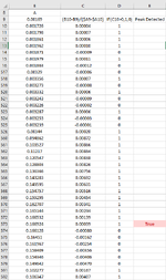
Here’s the main formula on Column E
=IFERROR(IF(((B10-B9)/($A9-$A10))>0,IF(AND((B9-B8)/($A8-$A9)>0,(B10-B8>=0.0006),(B11-B10<=-0.0006)),"True",""),""),"")

Columns C and D are not used in the formula, they only inform if the difference between adjacent row values are positive (peak rise) or negative (peak fall). Column D shows this in 1's (rise) and 0's (fall).

I’d like to account for all the consecutive peak rises (positive values on Column C) after a peak fall (negative values on Column C), and determine if the difference between the start of the peak rise and it’s fall is >=0.0006
At the same time, account for all consecutive peak falls (negative values) after a peak rise, and determine if the difference between the start of the peak fall and the start of the next peak rise is <=-0.0006
If both of these conditions are met, then report "True", as a peak was detected.

I hope this makes sense. Thank you all in advance for your time!

 

[Peter_SSs]

There is way too much manual typing to set that up to test. Please consider providing the sample data and expected results** in a form that we can easily copy to test with.

MrExcel has a tool called “XL2BB” that lets you post samples of your data that will allow us to copy/paste it to our Excel spreadsheets, so we can work with the same copy of data that you are. Instructions on using this tool can be found here: XL2BB Add-in

Note that there is also a "Test Here” forum on this board. This is a place where you can test using this tool (or any other posting techniques that you want to test) before trying to use those tools in your actual posts.

** I assume that the result shown in column E of your image is not correct, or at least is not the only correct result. When providing the sample data, don't put that formula in column E if it is not providing the result(s) that you want. Instead, manually enter the correct result(s) in column E and provide a written description of how you determine the result(s) manually.

 

[mejohn]

Hi Peter, sorry it took this long to reply, but I was out for a few days.

Column E uses the following formula to detect the presence of a peak.
=IFERROR(IF(((B5-B4)/($A4-$A5))>0,IF(AND((B4-B3)/($A3-$A4)>0,(B5-B3>=0.0006),(B6-B5<=-0.0006)),"True",""),""),"")

In order for a peak to be valid, absorbance will have to rise and fall by at least absolute(0.0006).

The current formula only takes into account absorbance values that are one or two wavelengths apart, when in fact the peak could have been rising for many wavelengths and the same with falling.
I'd like a formula to check the totality of the peak rise and peak fall, to determine if that total rise and fall is => absolute value of 0.0006.

The easiest way to see the data is to plot wavelength as x-axis and absorbance as y-axis.

I hope this helps.

Please see the minisheet data below.

Thank you!

book1.xlsx
	A	B	C	D	E
1	wavelength	absorbance			Peak Detected
2
3	500	0.002144
4	499	0.002131	-0.00001	0
5	498	0.001947	-0.00018	0
6	497	0.001983	0.00004	1
7	496	0.002171	0.00019	1
8	495	0.002227	0.00006	1
9	494	0.002186	-0.00004	0
10	493	0.002113	-0.00007	0
11	492	0.002027	-0.00009	0
12	491	0.002101	0.00007	1
13	490	0.002223	0.00012	1
14	489	0.002209	-0.00001	0
15	488	0.002131	-0.00008	0
16	487	0.002217	0.00009	1
17	486	0.002202	-0.00001	0
18	485	0.002223	0.00002	1
19	484	0.002308	0.00009	1
20	483	0.002361	0.00005	1
21	482	0.0023	-0.00006	0
22	481	0.002297	0.00000	0
23	480	0.002372	0.00008	1
24	479	0.002322	-0.00005	0
25	478	0.002332	0.00001	1
26	477	0.002393	0.00006	1
27	476	0.002356	-0.00004	0
28	475	0.002357	0.00000	1
29	474	0.002625	0.00027	1
30	473	0.002555	-0.00007	0
31	472	0.002438	-0.00012	0
32	471	0.002486	0.00005	1
33	470	0.002475	-0.00001	0
34	469	0.002473	0.00000	0
35	468	0.002649	0.00018	1
36	467	0.002759	0.00011	1
37	466	0.002703	-0.00006	0
38	465	0.002652	-0.00005	0
39	464	0.002671	0.00002	1
40	463	0.002682	0.00001	1
41	462	0.002678	0.00000	0
42	461	0.002611	-0.00007	0
43	460	0.002608	0.00000	0
44	459	0.002964	0.00036	1
45	458	0.003159	0.00020	1
46	457	0.003182	0.00002	1
47	456	0.003182	0.00000	0
48	455	0.00326	0.00008	1
49	454	0.00337	0.00011	1
50	453	0.003377	0.00001	1
51	452	0.00321	-0.00017	0
52	451	0.003212	0.00000	1
53	450	0.003323	0.00011	1
54	449	0.003322	0.00000	0
55	448	0.003285	-0.00004	0
56	447	0.003246	-0.00004	0
57	446	0.003297	0.00005	1
58	445	0.003409	0.00011	1
59	444	0.003431	0.00002	1
60	443	0.003466	0.00003	1
61	442	0.003437	-0.00003	0
62	441	0.003498	0.00006	1
63	440	0.003529	0.00003	1
64	439	0.003456	-0.00007	0
65	438	0.00343	-0.00003	0
66	437	0.003431	0.00000	1
67	436	0.003347	-0.00008	0
68	435	0.00329	-0.00006	0
69	434	0.003356	0.00007	1
70	433	0.003273	-0.00008	0
71	432	0.003332	0.00006	1
72	431	0.003243	-0.00009	0
73	430	0.003226	-0.00002	0
74	429	0.003287	0.00006	1
75	428	0.003253	-0.00003	0
76	427	0.003239	-0.00001	0
77	426	0.00344	0.00020	1
78	425	0.0035	0.00006	1
79	424	0.003533	0.00003	1
80	423	0.00356	0.00003	1
81	422	0.003641	0.00008	1
82	421	0.003766	0.00013	1
83	420	0.003939	0.00017	1
84	419	0.004079	0.00014	1
85	418	0.004317	0.00024	1
86	417	0.004519	0.00020	1
87	416	0.004825	0.00031	1
88	415	0.005063	0.00024	1
89	414	0.005535	0.00047	1
90	413	0.006076	0.00054	1
91	412	0.006791	0.00072	1
92	411	0.007479	0.00069	1
93	410	0.008406	0.00093	1
94	409	0.00961	0.00120	1
95	408	0.010932	0.00132	1
96	407	0.012587	0.00166	1
97	406	0.014521	0.00193	1
98	405	0.016774	0.00225	1
99	404	0.019588	0.00281	1
100	403	0.022861	0.00327	1
101	402	0.026754	0.00389	1
102	401	0.031052	0.00430	1
103	400	0.035927	0.00488	1
104	399	0.041523	0.00560	1
105	398	0.047611	0.00609	1
106	397	0.054352	0.00674	1
107	396	0.061686	0.00733	1
108	395	0.069353	0.00767	1
109	394	0.077698	0.00835	1
110	393	0.086138	0.00844	1
111	392	0.094862	0.00872	1
112	391	0.103527	0.00866	1
113	390	0.11217	0.00864	1
114	389	0.120547	0.00838	1
115	388	0.128803	0.00826	1
116	387	0.136366	0.00756	1
117	386	0.143283	0.00692	1
118	385	0.149595	0.00631	1
119	384	0.154757	0.00516	1
120	383	0.159295	0.00454	1
121	382	0.162707	0.00341	1
122	381	0.165144	0.00244	1
123	380	0.166532	0.00139	1
124	379	0.166924	0.00039	1	True
125	378	0.166128	-0.00080	0
126	377	0.16451	-0.00162	0
127	376	0.161967	-0.00254	0
128	375	0.158409	-0.00356	0
129	374	0.154346	-0.00406	0
130	373	0.149642	-0.00470	0
131	372	0.144418	-0.00522	0
132	371	0.138783	-0.00564	0
133	370	0.132928	-0.00586	0
134	369	0.126963	-0.00597	0
135	368	0.121051	-0.00591	0
136	367	0.115216	-0.00584	0
137	366	0.110305	-0.00491	0
138	365	0.106084	-0.00422	0
139	364	0.102589	-0.00350	0
140	363	0.100788	-0.00180	0
141	362	0.100611	-0.00018	0
142	361	0.102277	0.00167	1
143	360	0.106347	0.00407	1
144	359	0.113024	0.00668	1
145	358	0.122721	0.00970	1
146	357	0.135793	0.01307	1
147	356	0.152377	0.01658	1
148	355	0.172963	0.02059	1
149	354	0.19769	0.02473	1
150	353	0.227107	0.02942	1
151	352	0.260918	0.03381	1
152	351	0.300206	0.03929	1
153	350	0.345237	0.04503	1
154	349	0.39667	0.05143	1
155	348	0.455689	0.05902	1
156	347	0.52384	0.06815	1
157	346	0.602681	0.07884	1
158	345	0.696132	0.09345	1
159	344	0.808508	0.11238	1
Raw Data Combined

Cell Formulas
Range	Formula
C4:C159	C4	=(B4-B3)/($A3-$A4)
D4:D159	D4	=IF(C4>0,1,0)
E5:E159	E5	=IFERROR(IF(((B5-B4)/($A4-$A5))>0,IF(AND((B4-B3)/($A3-$A4)>0,(B5-B3>=0.0006),(B6-B5<=-0.0006)),"True",""),""),"")

Cells with Conditional Formatting
Cell	Condition		Cell Format	Stop If True
E:E	Cell Value	contains "True"	text	NO

 

[Peter_SSs]

Thanks for the XL2BB sample data.

Unfortunately, I should also have asked to you to manually insert the expected results. Anyway, this is my best guess, though particularly unsure how to handle things near the start and end of the data. If this is not it please remove your existing formulas from column E and manually add the expected results, repost that and explain why yours are the expected results.
I have hidden some of the middle rows as there were no True values from my formula there and it keeps the mini-sheet smaller for easier viewing in the forum.

mejohn.xlsm
	A	B	C	D	E
1	wavelength	absorbance
2
3	500	0.002144
4	499	0.002131	-0.000013	0
5	498	0.001947	-0.000184	0	True
6	497	0.001983	0.000036	1
7	496	0.002171	0.000188	1
8	495	0.002227	0.000056	1
9	494	0.002186	-0.000041	0
76	427	0.003239	-0.000014	0
77	426	0.00344	0.000201	1
78	425	0.0035	0.000060	1
79	424	0.003533	0.000033	1
80	423	0.00356	0.000027	1
81	422	0.003641	0.000081	1
82	421	0.003766	0.000125	1
83	420	0.003939	0.000173	1
84	419	0.004079	0.000140	1
85	418	0.004317	0.000238	1
86	417	0.004519	0.000202	1
87	416	0.004825	0.000306	1
88	415	0.005063	0.000238	1
89	414	0.005535	0.000472	1
90	413	0.006076	0.000541	1
91	412	0.006791	0.000715	1
92	411	0.007479	0.000688	1
93	410	0.008406	0.000927	1
94	409	0.00961	0.001204	1
95	408	0.010932	0.001322	1
96	407	0.012587	0.001655	1
97	406	0.014521	0.001934	1
98	405	0.016774	0.002253	1
99	404	0.019588	0.002814	1
100	403	0.022861	0.003273	1
101	402	0.026754	0.003893	1
102	401	0.031052	0.004298	1
103	400	0.035927	0.004875	1
104	399	0.041523	0.005596	1
105	398	0.047611	0.006088	1
106	397	0.054352	0.006741	1
107	396	0.061686	0.007334	1
108	395	0.069353	0.007667	1
109	394	0.077698	0.008345	1
110	393	0.086138	0.008440	1
111	392	0.094862	0.008724	1
112	391	0.103527	0.008665	1
113	390	0.11217	0.008643	1
114	389	0.120547	0.008377	1
115	388	0.128803	0.008256	1
116	387	0.136366	0.007563	1
117	386	0.143283	0.006917	1
118	385	0.149595	0.006312	1
119	384	0.154757	0.005162	1
120	383	0.159295	0.004538	1
121	382	0.162707	0.003412	1
122	381	0.165144	0.002437	1
123	380	0.166532	0.001388	1
124	379	0.166924	0.000392	1	True
125	378	0.166128	-0.000796	0
126	377	0.16451	-0.001618	0
127	376	0.161967	-0.002543	0
128	375	0.158409	-0.003558	0
129	374	0.154346	-0.004063	0
130	373	0.149642	-0.004704	0
131	372	0.144418	-0.005224	0
132	371	0.138783	-0.005635	0
133	370	0.132928	-0.005855	0
134	369	0.126963	-0.005965	0
135	368	0.121051	-0.005912	0
136	367	0.115216	-0.005835	0
137	366	0.110305	-0.004911	0
138	365	0.106084	-0.004221	0
139	364	0.102589	-0.003495	0
140	363	0.100788	-0.001801	0
141	362	0.100611	-0.000177	0	True
142	361	0.102277	0.001666	1
143	360	0.106347	0.004070	1
144	359	0.113024	0.006677	1
145	358	0.122721	0.009697	1
146	357	0.135793	0.013072	1
147	356	0.152377	0.016584	1
148	355	0.172963	0.020586	1
149	354	0.19769	0.024727	1
150	353	0.227107	0.029417	1
151	352	0.260918	0.033811	1
152	351	0.300206	0.039288	1
153	350	0.345237	0.045031	1
154	349	0.39667	0.051433	1
155	348	0.455689	0.059019	1
156	347	0.52384	0.068151	1
157	346	0.602681	0.078841	1
158	345	0.696132	0.093451	1
159	344	0.808508	0.112376	1	True
Sheet1

Cell Formulas
Range	Formula
C4:C9,C76:C159	C4	=(B4-B3)/($A3-$A4)
D4:D9,D76:D159	D4	=IF(C4>0,1,0)
E4:E9,E76:E159	E4	=IF(D4=D5,"",IF(ABS(XLOOKUP(D5,D$1:D3,B$1:B3,0,0,-1)-B4)>=0.0006,"True",""))

 

[mejohn]

Hi Peter,

Thank you for the new formula. It's very close to what I need.

I think the discrepancy is that your formula accounts for peak maximum and peak minimum. We're only looking for peak maximum.

Column D resolves to 0 or 1 based on whether Column C is negative or positive.
Column C will subtract current absorbance value - absorbance value of previous row.
If the value in Column C is negative, then absorbance is going down and the peak is falling.
If the value in Column C is positive, then absorbance is going up and the peak is rising.

You have "True" under peak detection for wavelength 498, 379, 362 and 343.

The only true peak maximum in the data is at wavelength 379, with an absorbance value of 0.166924.
That peak rose from wavelength 426 until 379 (consecutive 1's in Column D) and the total absorbance difference during the rise (B123-B76) is 0.163484, which is >=0.0006.
After peak maximum at 379, the peak falls from wavelength 378-362 and the total absorbance difference during the fall (B140-B124) is -0.06552, which is <=-0.0006.

Wavelength 498 and 362 can be considered peak minimums, but we're only need maximums.

Towards the end of the data wavelengths 361-343, the peak rises (1's in Column D), but never falls (no zeros after the rise) so we can't consider it a peak maximum.

I hope this better explains what I'm looking for.

Thank you so much for your time!

 

[Peter_SSs]

your formula accounts for peak maximum and peak minimum. We're only looking for peak maximum.

Hmm, I guess that I misinterpreted this then.

I’d like to account for all the consecutive peak rises ....
At the same time, account for all consecutive peak falls ....

The only true peak maximum in the data is at wavelength 379, with an absorbance value of 0.166924.

Why not wavelength 344 as well?

Is this closer? (Again, some rows hidden)

mejohn.xlsm
	A	B	C	D
1	wavelength	absorbance		Peak Detected
2
3	500	0.002144
4	499	0.002131	0
5	498	0.001947	0
6	497	0.001983	1
7	496	0.002171	2
8	495	0.002227	3
9	494	0.002186	0
73	430	0.003226	0
74	429	0.003287	1
75	428	0.003253	0
76	427	0.003239	0
77	426	0.00344	1
78	425	0.0035	2
79	424	0.003533	3
80	423	0.00356	4
81	422	0.003641	5
82	421	0.003766	6
83	420	0.003939	7
84	419	0.004079	8
85	418	0.004317	9
86	417	0.004519	10
87	416	0.004825	11
88	415	0.005063	12
89	414	0.005535	13
90	413	0.006076	14
91	412	0.006791	15
92	411	0.007479	16
93	410	0.008406	17
94	409	0.00961	18
95	408	0.010932	19
96	407	0.012587	20
97	406	0.014521	21
98	405	0.016774	22
99	404	0.019588	23
100	403	0.022861	24
101	402	0.026754	25
102	401	0.031052	26
103	400	0.035927	27
104	399	0.041523	28
105	398	0.047611	29
106	397	0.054352	30
107	396	0.061686	31
108	395	0.069353	32
109	394	0.077698	33
110	393	0.086138	34
111	392	0.094862	35
112	391	0.103527	36
113	390	0.11217	37
114	389	0.120547	38
115	388	0.128803	39
116	387	0.136366	40
117	386	0.143283	41
118	385	0.149595	42
119	384	0.154757	43
120	383	0.159295	44
121	382	0.162707	45
122	381	0.165144	46
123	380	0.166532	47
124	379	0.166924	48	True
125	378	0.166128	0
126	377	0.16451	0
140	363	0.100788	0
141	362	0.100611	0
142	361	0.102277	1
143	360	0.106347	2
144	359	0.113024	3
145	358	0.122721	4
146	357	0.135793	5
147	356	0.152377	6
148	355	0.172963	7
149	354	0.19769	8
150	353	0.227107	9
151	352	0.260918	10
152	351	0.300206	11
153	350	0.345237	12
154	349	0.39667	13
155	348	0.455689	14
156	347	0.52384	15
157	346	0.602681	16
158	345	0.696132	17
159	344	0.808508	18	True
Sheet3

Cell Formulas
Range	Formula
C4:C9,C73:C126,C140:C159	C4	=(C3+1)*(B4>B3)
D4:D9,D73:D126,D140:D159	D4	=IF(OR(C4=0,C5>0),"",IF(B4-XLOOKUP(1,C$1:C3,B$1:B3,0,0,-1)>=0.0006,"True",""))

 

[Peter_SSs]

Why not wavelength 344 as well?

On re-reading, I think that I should be looking down as well as up?

Another try to consider.

mejohn.xlsm
	A	B	C	D
1	wavelength	absorbance		Peak Detected
2
3	500	0.002144
4	499	0.002131	0
5	498	0.001947	0
6	497	0.001983	1
7	496	0.002171	2
8	495	0.002227	3
9	494	0.002186	0
73	430	0.003226	0
74	429	0.003287	1
75	428	0.003253	0
76	427	0.003239	0
77	426	0.00344	1
78	425	0.0035	2
79	424	0.003533	3
80	423	0.00356	4
81	422	0.003641	5
82	421	0.003766	6
83	420	0.003939	7
84	419	0.004079	8
85	418	0.004317	9
86	417	0.004519	10
87	416	0.004825	11
88	415	0.005063	12
89	414	0.005535	13
90	413	0.006076	14
91	412	0.006791	15
92	411	0.007479	16
93	410	0.008406	17
94	409	0.00961	18
95	408	0.010932	19
96	407	0.012587	20
97	406	0.014521	21
98	405	0.016774	22
99	404	0.019588	23
100	403	0.022861	24
101	402	0.026754	25
102	401	0.031052	26
103	400	0.035927	27
104	399	0.041523	28
105	398	0.047611	29
106	397	0.054352	30
107	396	0.061686	31
108	395	0.069353	32
109	394	0.077698	33
110	393	0.086138	34
111	392	0.094862	35
112	391	0.103527	36
113	390	0.11217	37
114	389	0.120547	38
115	388	0.128803	39
116	387	0.136366	40
117	386	0.143283	41
118	385	0.149595	42
119	384	0.154757	43
120	383	0.159295	44
121	382	0.162707	45
122	381	0.165144	46
123	380	0.166532	47
124	379	0.166924	48	True
125	378	0.166128	0
126	377	0.16451	0
140	363	0.100788	0
141	362	0.100611	0
142	361	0.102277	1
143	360	0.106347	2
144	359	0.113024	3
145	358	0.122721	4
146	357	0.135793	5
147	356	0.152377	6
148	355	0.172963	7
149	354	0.19769	8
150	353	0.227107	9
151	352	0.260918	10
152	351	0.300206	11
153	350	0.345237	12
154	349	0.39667	13
155	348	0.455689	14
156	347	0.52384	15
157	346	0.602681	16
158	345	0.696132	17
159	344	0.808508	18
Sheet4

Cell Formulas
Range	Formula
C4:C9,C73:C126,C140:C159	C4	=(C3+1)*(B4>B3)
D4:D9,D73:D126,D140:D159	D4	=IF(OR(C4=0,C5>0),"",IF(MIN(B4-XLOOKUP(1,C$1:C3,B$1:B3,0,0,-1),B4-XLOOKUP(1,C5:C$160,B4:B$159,B4))>=0.0006,"True",""))

 

[mejohn]

Hi Peter,

This data represents a UV-Vis scan that starts at high wavelength number say 500, down to lower wavelength 344.
As the scan progresses, if there's a peak maximum, absorbance will increase until peak maximum, then absorbance will decrease.
This increase and decrease of absorbance can be over multiple consecutive wavelengths.
Before and after peak maximums, there can be noise (absorbance increases and decreases, but not sufficient to overcome the instrument's sensitivity of abs(0.0006) for both the rise and the fall of the peak)
Therefore, a peak maximum has to be defined by not only and increase in absorbance, but also followed by a decrease in absorbance that is greater than the instrument sensitivity.
Wavelength 344 is not a peak maximum since it is not followed by decreasing absorbance.
The scan ended at 344. If the scan would have continued to say 300nm, there may have been a peak maximum somewhere between 344-300nm, but we don't know for sure. There are multiple reasons to limit the range of the scan.

The formula is almost perfect.

I did find an issue when trying it out on another scan, where the peak rises until the next to last wavelength and then drops in the last wavelength by <=-0.0006 (new data B99-B98), but the formula does not detect the peak maximum.
Maybe because it's the end of the data.

Please see data below.

Thank so much!

book2.xlsx
	A	B	C	D
1	Wavelength (nm)	A		Peak Detected
2	500	0.000056
3	499	0.000071	1
4	498	-0.000063	0
5	497	-0.000075	0
6	496	-0.000182	0
7	495	-0.000157	1
8	494	-0.000137	2
9	493	-0.00009	3
10	492	-0.000064	4
11	491	-0.000045	5
12	490	-0.000043	6
13	489	-0.00005	0
14	488	-0.000002	1
15	487	-0.000106	0
16	486	-0.00004	1
17	485	0.000065	2
18	484	-0.000018	0
19	483	0.000084	1
20	482	-0.000017	0
21	481	-0.000015	1
22	480	0	2
23	479	-0.000045	0
24	478	0.000051	1
25	477	0.00004	0
26	476	0.000052	1
27	475	0.000154	2
28	474	0.00024	3
29	473	0.000393	4
30	472	0.00057	5
31	471	0.000909	6
32	470	0.001472	7
33	469	0.002217	8
34	468	0.00356	9
35	467	0.00599	10
36	466	0.010754	11
37	465	0.017665	12
38	464	0.024182	13
39	463	0.026645	14	True
40	462	0.025708	0
41	461	0.024894	0
42	460	0.024955	1
43	459	0.025687	2
44	458	0.028208	3
45	457	0.031899	4
46	456	0.03434	5
47	455	0.034612	6	True
48	454	0.033498	0
49	453	0.031312	0
50	452	0.028894	0
51	451	0.027435	0
52	450	0.026936	0
53	449	0.026521	0
54	448	0.025438	0
55	447	0.02361	0
56	446	0.021453	0
57	445	0.019494	0
58	444	0.018006	0
59	443	0.01668	0
60	442	0.014991	0
61	441	0.013199	0
62	440	0.011388	0
63	439	0.0099	0
64	438	0.008593	0
65	437	0.007228	0
66	436	0.005909	0
67	435	0.004428	0
68	434	0.003003	0
69	433	0.001809	0
70	432	0.000637	0
71	431	-0.000505	0
72	430	-0.001607	0
73	429	-0.002658	0
74	428	-0.003475	0
75	427	-0.004088	0
76	426	-0.004466	0
77	425	-0.004258	1
78	424	-0.003262	2
79	423	-0.00098	3
80	422	0.003508	4
81	421	0.011929	5
82	420	0.026353	6
83	419	0.049481	7
84	418	0.084763	8
85	417	0.135364	9
86	416	0.203233	10
87	415	0.288077	11
88	414	0.384543	12
89	413	0.488092	13
90	412	0.601672	14
91	411	0.729055	15
92	410	0.861495	16
93	409	0.977181	17
94	408	1.059937	18
95	407	1.118963	19
96	406	1.165861	20
97	405	1.200559	21
98	404	1.214909	22	peak maximum
99	403	1.213558	0
Raw Data Combined

Cell Formulas
Range	Formula
D3:D97	D3	=IF(OR(C3=0,C4>0),"",IF(MIN(B3-XLOOKUP(1,C$2:C2,B$2:B2,0,0,-1),B3-XLOOKUP(1,C4:C$99,B3:B$98,B3))>=0.0006,"True",""))
C3:C99	C3	=(C2+1)*(B3>B2)
D99	D99	=IF(OR(C99=0,C100>0),"",IF(MIN(B99-XLOOKUP(1,C$2:C98,B$2:B98,0,0,-1),B99-XLOOKUP(1,C$99:C100,B$98:B99,B99))>=0.0006,"True",""))

Cells with Conditional Formatting
Cell	Condition		Cell Format	Stop If True
D1	Cell Value	contains "TRUE"	text	NO
D1	Cell Value	="TEXT"	text	NO
D2:D1048576,G3:G1048576,J3:J1048576	Cell Value	contains "True"	text	NO

 

[mejohn]

Sorry, there are three peak maximums in this data.
Wavelengths 463, 455, 404.
Thank you!

 

[Peter_SSs]

Try

mejohn.xlsm
	A	B	C	D
1	Wavelength (nm)	A		Peak Detected
2	500	0.000056
3	499	0.000071	1
4	498	-0.000063	0
5	497	-0.000075	0
6	496	-0.000182	0
7	495	-0.000157	1
23	479	-0.000045	0
24	478	0.000051	1
25	477	0.00004	0
26	476	0.000052	1
27	475	0.000154	2
28	474	0.00024	3
29	473	0.000393	4
30	472	0.00057	5
31	471	0.000909	6
32	470	0.001472	7
33	469	0.002217	8
34	468	0.00356	9
35	467	0.00599	10
36	466	0.010754	11
37	465	0.017665	12
38	464	0.024182	13
39	463	0.026645	14	True
40	462	0.025708	0
41	461	0.024894	0
42	460	0.024955	1
43	459	0.025687	2
44	458	0.028208	3
45	457	0.031899	4
46	456	0.03434	5
47	455	0.034612	6	True
48	454	0.033498	0
49	453	0.031312	0
76	426	-0.004466	0
77	425	-0.004258	1
78	424	-0.003262	2
79	423	-0.00098	3
80	422	0.003508	4
81	421	0.011929	5
82	420	0.026353	6
83	419	0.049481	7
84	418	0.084763	8
85	417	0.135364	9
86	416	0.203233	10
87	415	0.288077	11
88	414	0.384543	12
89	413	0.488092	13
90	412	0.601672	14
91	411	0.729055	15
92	410	0.861495	16
93	409	0.977181	17
94	408	1.059937	18
95	407	1.118963	19
96	406	1.165861	20
97	405	1.200559	21
98	404	1.214909	22	True
99	403	1.213558	0
Sheet2

Cell Formulas
Range	Formula
C3:C7,C23:C49,C76:C99	C3	=(C2+1)*(B3>B2)
D3:D7,D23:D49,D76:D99	D3	=IF(OR(C3=0,C4>0),"",IF(MIN(B3-XLOOKUP(1,C$2:C2,B$2:B2,0,0,-1),B3-XLOOKUP(1,C4:C$100,B3:B$99,B$99))>=0.0006,"True",""))