Determine if a date falls between two dates in Excel and Return a number value in another colum

[cwallace70]

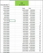
I have column A with specific dates, Column B with start dates, column C with end dates, and column C with a value.
I need a formula to look at the date in column A determine where it falls between the start and end dates in columns B & C and return the number value in column C.

 

[RoryA]

You can use something like (I've assumed the lookup table is actually columns B:D on another sheet, not columns B, C and C again):

=LOOKUP(1/((Sheet2!$B$2:$B$1000<=A2)*(Sheet2!$C$2:$C$1000>=A2)),Sheet2!$D$2:$D$1000)

 

[cwallace70]

You can use something like (I've assumed the lookup table is actually columns B:D on another sheet, not columns B, C and C again):

=LOOKUP(1/((Sheet2!$B$2:$B$1000<=A2)*(Sheet2!$C$2:$C$1000>=A2)),Sheet2!$D$2:$D$1000)

Yes, everything is on one sheet. Correction is Column D and not C again

 

[cwallace70]

=LOOKUP(1/((@$B$2:$B$1000<=A3)*(@$C$2:$C$1000>=A3)),$D$2:$D$1000) IS GIVING ME A #DIV/0! ERROR MESSAGE.

 

[RoryA]

Remove the @ symbols

 

[cwallace70]

I removed the @ symbol now I am getting the #SPILL! error message
=LOOKUP(1/(($T$3:$T$26>=G2)*($U$3:$U$26<=G2)),$V$3:$V$26)

 

[Alex Blakenburg]

I removed the @ symbol now I am getting the #SPILL! error message
=LOOKUP(1/(($T$3:$T$26>=G2)*($U$3:$U$26<=G2)),$V$3:$V$26)

Giving different column references in the initial enquiry then what you are actually using just complicates the exercise.
The way you have your column T and U referenced assumes that
- T is the End Date and
- U is the Start Date
(this reverses the original order)
If this is correct then try this:-

=LOOKUP(2,1/(($T$3:$T$26>=G2)*($U$3:$U$26<=G2)),$V$3:$V$26)

If you have mistakenly inverted the order in changing the column references to your real column references and
- T is the Start Date and
- U is the End Date
then try this:-

=LOOKUP(2,1/(($U$3:$U$26>=G2)*($T$3:$T$26<=G2)),$V$3:$V$26)

 

[RoryA]

Apologies - I missed out the 2, part at the start of the formula!

 

[cwallace70]

This formula worked?. Thank you. This has eliminated a manual time-consuming process. I appreciate it!

=LOOKUP(2,1/(($U$3:$U$26>=G2)*($T$3:$T$26<=G2)),$V$3:$V$26)

 

[Alex Blakenburg]

Glad we could help & thank you for the feedback. I especially appreciate that you clarified which option ended up working for you.