Display name of highest score on a particular date

MrNoobster

New Member
Joined
Dec 18, 2019
Messages
10
Office Version
  1. 2010
Platform
  1. Windows
Good Evening All,

I have myself a customised version of the below formula which gives me the information I require, however I would like to add in date.
So as per the example below, we have Thomas who scored 128. I want it to read Thomas scored 128 on (date). The date would be on a range of cells but I'm not sure where to add this into the corresponding formula.

My formula is =INDEX(B18:B3000,MATCH(MAX(AB18:AB3000),AB18:AB3000,FALSE),)&" with "&MAX(AB18:AB3000)&" trailer moves on " I want to add "on (specific date in a range of cells that correspond to the name)


Can anyone help?

Many thanks


Please enter this formula: =INDEX(A2:A14,MATCH(MAX(B2:B14),B2:B14,FALSE),)&" Scored "&MAX(B2:B14) into a blank cell where you want to display the name, and then press Enter key to return the result as follows:
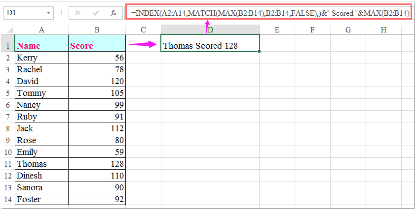
doc display name highest score 1
 

Excel Facts

Easy bullets in Excel
If you have a numeric keypad, press Alt+7 on numeric keypad to type a bullet in Excel.
Wouldn't it be possible for more than one person to have equal highest score on a particular date?
If so, you could try this formula, copied down.

Book1
ABCDEF
1NameDateScoreDateName(s)
2Name 1622/09/20174224/09/2017Name 10
3Name 2922/09/201774Name 28
4Name 4622/09/201740 
5Name 222/09/201762 
6Name 7822/09/201752
7Name 4323/09/201742
8Name 6923/09/201777
9Name 5624/09/201767
10Name 1024/09/201780
11Name 5824/09/201778
12Name 2824/09/201780
13Name 7224/09/201773
14Name 3225/09/201748
15Name 7125/09/201746
16Name 7525/09/201765
17Name 3525/09/201744
18Name 6425/09/201780
19Name 6225/09/201744
20
High Score on Date
Cell Formulas
RangeFormula
F2:F5F2=IFERROR(INDEX(A:A,AGGREGATE(15,6,ROW(A$2:A$19)/((B$2:B$19=E$2)*(C$2:C$19=AGGREGATE(14,6,C$2:C$19/(B$2:B$19=E$2),1))),ROWS(F$2:F2))),"")
 
Upvote 0
.. or perhaps like this

Book1
ABCDEFG
1NameDateScoreDateMax for dateName(s)
2Name 1622/09/20174224/09/201780Name 10
3Name 2922/09/201774Name 28
4Name 4622/09/201740 
5Name 222/09/201762 
6Name 7822/09/201752
7Name 4323/09/201742
8Name 6923/09/201777
9Name 5624/09/201767
10Name 1024/09/201780
11Name 5824/09/201778
12Name 2824/09/201780
13Name 7224/09/201773
14Name 3225/09/201748
15Name 7125/09/201746
16Name 7525/09/201765
17Name 3525/09/201744
18Name 6425/09/201780
19Name 6225/09/201744
20
High Score on Date
Cell Formulas
RangeFormula
F2F2=AGGREGATE(14,6,C2:C19/(B2:B19=E2),1)
G2:G5G2=IFERROR(INDEX(A:A,AGGREGATE(15,6,ROW(A$2:A$19)/((B$2:B$19=E$2)*(C$2:C$19=F$2)),ROWS(G$2:G2))),"")
 
Upvote 0
Hi Peter, and thanks for your reply. I don't think I explained what i needed very well however that formula is useful for something else I'm working on so I thank you for that. I'll try to be a bit more specific with my actual data:

I have this table:
NameTotal Moves to DateTotal Shunt Hours% of MovesMoves per hourNumber of Shifts% of Shifts
Ollie Calcott35610447.28%3.421431.82%
Mark Whitehead65488.63%1.35613.64%
Alan Smith834811.02%1.73613.64%
Kai Fluke1278816.87%1.441125.00%
Nigel Southwood59197.84%3.1124.55%
Mark Wagstaff000.00%#DIV/0!00.00%
Bernard Coyle000.00%#DIV/0!00.00%
Wayne Smith1081.33%1.2512.27%
John Black53327.04%1.6649.09%
Arek Dregier000.00%#DIV/0!00.00%
Thomas Mulvany000.00%#DIV/0!00.00%


What i'm trying to create is a cell which states simply that (name) with (number) trailer moves on (date).

At the moment it looks like this:
Most moves on a single shift:
Nigel Southwood with 51 trailer moves on

The cell that says "Nigel Southwood with 51 trailer moves on" has the following formula:

=INDEX(B18:B3001,MATCH(MAX(AB18:AB3001),AB18:AB3001,FALSE),)&" with "&MAX(AB18:AB3001)&" trailer moves on "

I have a separate column with dates corresponding to the trailer moves a driver has completed, which is A18:A3000.

I would like the cell to read "Nigel Southwood with 51 trailer moves on Monday 6th January" so with the original formula I believe something needs adding to it to make that happen but I can't wrap my brain around it.

Many thanks in advance
 
Upvote 0
What rows and columns have you shown us there? (would be clearer if you could use XL2BB like I did above. ;))

And what relationship does that sample data have to getting the result? I can't see 51 anywhere in that data & I can't see any dates. Don't we need to be able to see a small sample of columns A and AB and how they relate to this shown data and/or the actual result required? Those columns are used in your formula but from what I can tell they are not part of the table you have shown.

Also, isn't my previous question still valid? Isn't it 'possible' for the maximum value in column AB to occur on more than one row of column AB?
 
Upvote 0
Hi Peter,

Thanks for the advice, I've just installed XL2BB...please see below. I apologise if it looks messy but I'm still rather new to posting on forums. This is my entire front sheet which generates information on other tabs however this is my master tab.

Book1
ABCDEFGHIJKLMNOPQRSTUVWXYZAAABAC
1NameTotal Moves to DateTotal Shunt Hours% of MovesMoves per hourNumber of Shifts% of ShiftsMost moves on a single shift:07:00 - 15:00
2Ollie Calcott35610447.28%3.421431.82%Nigel Southwood with 51 trailer moves on 22:00 - 06:00
3Mark Whitehead65488.63%1.35613.64%06:00 - 14:00
4Alan Smith834811.02%1.73613.64%14:00 - 22:00
5Kai Fluke1278816.87%1.441125.00%YTD AVG Hourly Trailer Moves15:00 - 22:00
6Nigel Southwood59197.84%3.1124.55%
7Mark Wagstaff000.00%#DIV/0!00.00%00:00 - 01:0001:00 - 02:0002:00 - 03:0003:00 - 04:0004:00 - 05:0005:00 - 06:0006:00 - 07:0007:00 - 08:0008:00 - 09:0009:00 - 10:0010:00 - 11:0011:00 - 12:0012:00 - 13:0013:00 - 14:0014:00 - 15:0015:00 - 16:0016:00 - 17:0017:00 - 18:0018:00 - 19:0019:00 - 20:0020:00 - 21:0021:00 - 22:00
8Bernard Coyle000.00%#DIV/0!00.00%3.802.872.733.003.642.642.001.632.381.001.630.881.131.190.500.751.771.460.922.922.622.85
9Wayne Smith1081.33%1.2512.27%
10John Black53327.04%1.6649.09%YTD Total Trailer Moves
11Arek Dregier000.00%#DIV/0!00.00%00:00 - 01:0001:00 - 02:0002:00 - 03:0003:00 - 04:0004:00 - 05:0005:00 - 06:0006:00 - 07:0007:00 - 08:0008:00 - 09:0009:00 - 10:0010:00 - 11:0011:00 - 12:0012:00 - 13:0013:00 - 14:0014:00 - 15:0015:00 - 16:0016:00 - 17:0017:00 - 18:0018:00 - 19:0019:00 - 20:0020:00 - 21:0021:00 - 22:00
12Thomas Mulvany000.00%#DIV/0!00.00%574341425137322638162614181969231912383437
1375334744
14
15
16
17DateShunterShift00:00 - 01:0001:00 - 02:0002:00 - 03:0003:00 - 04:0004:00 - 05:0005:00 - 06:0006:00 - 07:0007:00 - 08:0008:00 - 09:0009:00 - 10:0010:00 - 11:0011:00 - 12:0012:00 - 13:0013:00 - 14:0014:00 - 15:0015:00 - 16:0016:00 - 17:0017:00 - 18:0018:00 - 19:0019:00 - 20:0020:00 - 21:0021:00 - 22:0022:00 - 23:0023:00 - 00:00Total moves for shiftTotal shift time
18Wednesday 1st JanuaryOllie Calcott22:00 - 06:0062420871308
19Thursday 2nd JanuaryAlan Smith06:00 - 14:0048022002188
20Thursday 2nd JanuaryMark Whitehead14:00 - 22:0004020104118
21Thursday 2nd JanuaryOllie Calcott22:00 - 06:00009527101348
22Friday 3rd JanuaryAlan Smith06:00 - 14:0022407301198
23Friday 3rd JanuaryMark Whitehead14:00 - 22:000000051178
24Saturday 4th JanuaryMark Whitehead06:00 - 14:0043020327218
25Sunday 5th JanuaryOllie Calcott22:00 - 06:0051105114188
26Monday 6th JanuaryKai Fluke06:00 - 14:000001200038
27Monday 6th JanuaryMark Whitehead14:00 - 22:0002305010118
28Monday 6th JanuaryOllie Calcott22:00 - 06:00140264247398
29Tuesday 7th JanuaryKai Fluke06:00 - 14:000000403078
30Tuesday 7th JanuaryAlan Smith14:00 - 22:0010042434188
31Tuesday 7th JanuaryOllie Calcott22:00 - 06:0030227188318
32Wednesday 8th JanuaryKai Fluke06:00 - 14:0003304002128
33Wednesday 8th JanuaryAlan Smith14:00 - 22:0010420423168
34Wednesday 8th JanuaryOllie Calcott22:00 - 06:0024035245258
35Thursday 9th JanuaryKai Fluke06:00 - 14:0000600050118
36Thursday 9th JanuaryAlan Smith14:00 - 22:001010003058
37Thursday 9th JanuaryOllie Calcott22:00 - 06:00224460713388
38Friday 10th JanuaryKai Fluke06:00 - 14:0000800300118
39Friday 10th JanuaryAlan Smith14:00 - 22:000020203078
40Friday 10th JanuaryNigel Southwood22:00 - 06:001311002088
41Saturday 11th JanuaryMark Whitehead06:00 - 14:0041050020128
42Sunday 12th JanuaryOllie Calcott22:00 - 06:0032113090198
43Monday 13th JanuaryMark Whitehead06:00 - 14:000030000038
44Monday 13th JanuaryKai Fluke14:00 - 22:0002200512128
45Monday 13th JanuaryOllie Calcott22:00 - 06:00910062720368
46Tuesday 14th JanuaryJohn Black07:00 - 15:0013016133188
47Tuesday 14th JanuaryKai Fluke14:00 - 22:0000050247188
48Tuesday 14th JanuaryOllie Calcott22:00 - 06:0012246443268
49Wednesday 15th JanuaryJohn Black07:00 - 15:0051500130158
50Wednesday 15th JanuaryKai Fluke14:00 - 22:0001400212108
51Wednesday 15th JanuaryOllie Calcott22:00 - 06:0042020424188
52Thursday 16th JanuaryJohn Black07:00 - 15:0041320000108
53Thursday 16th JanuaryKai Fluke14:00 - 22:0020300452168
54Thursday 16th JanuaryOllie Calcott22:00 - 06:0006607005248
55Friday 17th JanuaryJohn Black07:00 - 15:0070020100108
56Friday 17th JanuaryKai Fluke14:00 - 22:0010150605188
57Saturday 18th JanuaryWayne Smith06:00 - 14:0012311002108
58Sunday 19th JanuaryOllie Calcott22:00 - 06:0030264102188
59Monday 20th JanuaryKai Fluke06:00 - 14:000230020298
60Monday 20th JanuaryNigel Southwood16:00 - 03:004973135107205111
61Monday 20th JanuaryOllie Calcott03:00 - 06:0000
Master
Cell Formulas
RangeFormula
B2B2=SUMIF(B18:B3003,A2,AB18:AB3003)
C2C2=SUMIF(B18:B3003,A2,AC18:AC3003)
D2D2=B2/SUM(B2:B12)
E2:E12E2=B2/C2
B3B3=SUMIF(B18:B3003,A3,AB18:AB3003)
C3C3=SUMIF(B18:B3003,A3,AC18:AC3003)
D3D3=B3/SUM(B2:B12)
B4B4=SUMIF(B18:B3003,A4,AB18:AB3003)
C4C4=SUMIF(B18:B3003,A4,AC18:AC3003)
D4D4=B4/SUM(B2:B12)
B5B5=SUMIF(B18:B3003,A5,AB18:AB3003)
C5C5=SUMIF(B18:B3003,A5,AC18:AC3003)
D5D5=B5/SUM(B2:B12)
B6B6=SUMIF(B18:B3003,A6,AB18:AB3003)
C6C6=SUMIF(B18:B3003,A6,AC18:AC3003)
D6D6=B6/SUM(B2:B12)
B7B7=SUMIF(B18:B3003,A7,AB18:AB3003)
C7C7=SUMIF(B18:B3003,A7,AC18:AC3003)
D7D7=B7/SUM(B2:B12)
B8B8=SUMIF(B18:B3003,A8,AB18:AB3003)
C8C8=SUMIF(B18:B3003,A8,AC18:AC3003)
D8D8=B8/SUM(B2:B12)
B9B9=SUMIF(B18:B3003,A9,AB18:AB3003)
C9C9=SUMIF(B18:B3003,A9,AC18:AC3003)
D9D9=B9/SUM(B2:B12)
B10B10=SUMIF(B18:B3003,A10,AB18:AB3003)
C10C10=SUMIF(B18:B3003,A10,AC18:AC3003)
D10D10=B10/SUM(B2:B12)
B11B11=SUMIF(B18:B3003,A11,AB18:AB3003)
C11C11=SUMIF(B18:B3003,A11,AC18:AC3003)
D11D11=B11/SUM(B2:B12)
B12B12=SUMIF(B18:B3003,A12,AB18:AB3003)
C12C12=SUMIF(B18:B3003,A12,AC18:AC3003)
D12D12=B12/SUM(B2:B12)
J2J2=INDEX(B18:B3001,MATCH(MAX(AB18:AB3001),AB18:AB3001,FALSE),)&" with "&MAX(AB18:AB3001)&" trailer moves on "
H8:AC8H8=AVERAGE(D18:D3003)
G2G2=F2/SUM(F2:F12)
G3G3=F3/SUM(F2:F12)
G4G4=F4/SUM(F2:F12)
G5G5=F5/SUM(F2:F12)
G6G6=F6/SUM(F2:F12)
G7G7=F7/SUM(F2:F12)
G8G8=F8/SUM(F2:F12)
G9G9=F9/SUM(F2:F12)
G10G10=F10/SUM(F2:F12)
G11G11=F11/SUM(F2:F12)
G12G12=F12/SUM(F2:F12)
H12:AC12H12=SUM(D18:D3003)
B13:C13, F13B13=SUM(B2:B12)
F2F2=COUNTIF(B18:B3002,A2)
F3F3=COUNTIF(B18:B3002,A3)
F4F4=COUNTIF(B18:B3002,A4)
F5F5=COUNTIF(B18:B3002,A5)
F6F6=COUNTIF(B18:B3002,A6)
F7F7=COUNTIF(B18:B3002,A7)
F8F8=COUNTIF(B18:B3002,A8)
F9F9=COUNTIF(B18:B3002,A9)
F10F10=COUNTIF(B18:B3002,A10)
F11F11=COUNTIF(B18:B3002,A11)
F12F12=COUNTIF(B18:B3002,A12)
AB18:AB61AB18=SUM(D18:AA18)
AC18:AC61AC18=COUNT(D18:AA18)
Cells with Conditional Formatting
CellConditionCell FormatStop If True
E2:E12Cell Valuetop 1 bottom valuestextNO
E2:E12Cell Valuetop 1 valuestextNO
D2:D12Cell Valuetop 1 bottom valuestextNO
D2:D12Cell Valuetop 1 valuestextNO
B2:B12Cell Valuetop 1 bottom valuestextNO
B2:B12Cell Valuetop 1 valuestextNO
G2:G12Cell Valuetop 1 bottom valuestextNO
G2:G12Cell Valuetop 1 valuestextNO
F2:F12Cell Valuetop 1 bottom valuestextNO
F2:F12Cell Valuetop 1 valuestextNO
C2:C12Cell Valuetop 1 bottom valuestextNO
C2:C12Cell Valuetop 1 valuestextNO
Cells with Data Validation
CellAllowCriteria
B18:B61List=$A$2:$A$12
C18:C59List=$N$1:$N$5
 
Upvote 0
Thanks.
So in that example, you want this result in J2?
Nigel Southwood with 51 trailer moves on Monday 20th January

If so, and assuming the dates in column A are text and not actual dates, try adding this to the end of your formula.
=INDEX(B18:B3001,MATCH(MAX(AB18:AB3001),AB18:AB3001,FALSE),)&" with "&MAX(AB18:AB3001)&" trailer moves on "&INDEX(A18:A3001,MATCH(MAX(AB18:AB3001),AB18:AB3001,FALSE),)


However, you still haven't addressed the question I have asked twice already
Isn't it 'possible' for the maximum value in column AB to occur on more than one row of column AB?
For example, in that sample file, change X28 and Y28 to 6. Then ..

Nigel Southwood with 51 trailer moves on Monday 20th January
and
Ollie Calcott with 51 trailer moves on Monday 6th January

What result(s) do you want in that circumstance?
 
Upvote 0
Hi Peter,


That's done it, thank you so much!

Sorry for not answering your question twice, i was just concentrating on the current problem rather than thinking ahead to the next. Yes it is indeed possible for 2 or more people to have the same result.

The result I would like is exactly how you've portrayed it here
Nigel Southwood with 51 trailer moves on Monday 20th January
and
Ollie Calcott with 51 trailer moves on Monday 6th January

However again, I'm not sure how I would go about this. I don't understand your reference to changing X28 and Y28 to 6. Could you explain this please?


Many thanks
 
Upvote 0
The result I would like is exactly how you've portrayed it here
Excel 2010 does not lend itself to a process like that if you wanted multiple results in a single cell. We can do it if it is okay to produce each of the multiple results in its own cell. Is that acceptable?

I don't understand your reference to changing X28 and Y28 to 6. Could you explain this please?
I was just suggesting physically changing those 2 cells on the sample sheet (I've shown them yellow). That way, Ollie Calcott also ended up with 51 moves for the shift. So I was just forcing an example where the maximum value in AB occurred twice (blue cells). :)

Book1
ABCDEFGHIJWXYZAAAB
28Monday 6th JanuaryOllie Calcott22:00 - 06:001402642664751
60Monday 20th JanuaryNigel Southwood16:00 - 03:0049751072051
High Score on Date (2)
Cell Formulas
RangeFormula
AB28, AB60AB28=SUM(D28:AA28)
 
Upvote 0
Peter, you've been incredibly helpful and I can't thank you or this forum enough. Thank you so much for all your time and effort with this :)
 
Upvote 0

Forum statistics

Threads
1,214,520
Messages
6,120,013
Members
448,935
Latest member
ijat

We've detected that you are using an adblocker.

We have a great community of people providing Excel help here, but the hosting costs are enormous. You can help keep this site running by allowing ads on MrExcel.com.
Allow Ads at MrExcel

Which adblocker are you using?

Disable AdBlock

Follow these easy steps to disable AdBlock

1)Click on the icon in the browser’s toolbar.
2)Click on the icon in the browser’s toolbar.
2)Click on the "Pause on this site" option.
Go back

Disable AdBlock Plus

Follow these easy steps to disable AdBlock Plus

1)Click on the icon in the browser’s toolbar.
2)Click on the toggle to disable it for "mrexcel.com".
Go back

Disable uBlock Origin

Follow these easy steps to disable uBlock Origin

1)Click on the icon in the browser’s toolbar.
2)Click on the "Power" button.
3)Click on the "Refresh" button.
Go back

Disable uBlock

Follow these easy steps to disable uBlock

1)Click on the icon in the browser’s toolbar.
2)Click on the "Power" button.
3)Click on the "Refresh" button.
Go back
Back
Top