Displaying Multiple Matches in Complex Matrix

[CodyWoodman]

Hello,

I apologize if this question has been answered before, but I honestly have no idea what to search for.

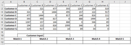
I have a matrix, where all the rows in column A are our customers' names. In row 1, I have a duplicate of all of our customers' names (the Matrix runs from A1:FF149). Each of the cells in the table has the distance between each customer in KM.

Essentially my goal is when a Customer's name is inputted, Excel will display other customers within a certain distance (say 200km).

I have posted a photo with a much smaller scale of what I'm trying to accomplish to give you an idea.

 

[shift-del]

Hi Cody

Change you data from crosstabular format into list format.

Mappe7
	J	K	L
2	A	B	167
3	A	C	322
4	A	D	100
5	A	E	121
6	B	C	443
7	B	D	271
8	B	E	243
9	C	D	242
10	C	E	130
11	D	E	362
12
13	B
14
15	A	167
16	E	243
17	D	271
Tabelle1

Cell Formulas
Range	Formula
J15:K17	J15	=SORT(TEXTSPLIT(TEXTJOIN({":";"|"},TRUE,FILTER(SUBSTITUTE(J2:L11,J13,""),((J2:J11=J13)+(K2:K11=J13))*(L2:L11<300))),":","|"),2)
Dynamic array formulas.

I used 5 functions. I wonder if less is possible.

 

[shift-del]

The original setup requires 7 functions.

Mappe7
	A	B	C	D	E	F
1		A	B	C	D	E
2	A		167	322	100	121
3	B	167		443	271	243
4	C	322	443		242	130
5	D	100	271	242		362
6	E	121	243	130	362
7
8
9		B
10
11		A	167
12		E	243
13		D	271
Tabelle1

Cell Formulas
Range	Formula
B11:C13	B11	=LET( a,HSTACK(A2:A6,INDEX(B2:F6,0,MATCH(B9,$B$1:$F$1,0))), b,INDEX(a,,2), c,FILTER(a,(b>0)*(b<300)), SORT(c,2))
Dynamic array formulas.

 

[Peter_SSs]

Welcome to the MrExcel board!

A slightly different version that you could also consider.

CodyWoodman.xlsm
	A	B	C	D	E	F	G
1		A	B	C	D	E
2	A		167	322	100	121
3	B	167		443	171	143
4	C	322	443		242	130
5	D	100	171	242		362
6	E	121	143	130	362
7
8
9		B
10
11		E	143
12		A	167
13		D	171
14
Sheet1

Cell Formulas
Range	Formula
B11:C13	B11	=LET(f,FILTER(A2:F6,(A1:F1=B9)+(A1:F1="")),d,INDEX(f,,2),SORT(FILTER(f,(d<200)*(d>0),{"",""}),2))
Dynamic array formulas.

 

[CodyWoodman]

The original setup requires 7 functions.

Mappe7
	A	B	C	D	E	F
1		A	B	C	D	E
2	A		167	322	100	121
3	B	167		443	271	243
4	C	322	443		242	130
5	D	100	271	242		362
6	E	121	243	130	362
7
8
9		B
10
11		A	167
12		E	243
13		D	271
Tabelle1

Cell Formulas
Range	Formula
B11:C13	B11	=LET( a,HSTACK(A2:A6,INDEX(B2:F6,0,MATCH(B9,$B$1:$F$1,0))), b,INDEX(a,,2), c,FILTER(a,(b>0)*(b<300)), SORT(c,2))
Dynamic array formulas.

This worked for me perfectly!!! Thank you!!