Divided set of data by choice in Sequence

ivanlost

New Member
Joined
Feb 22, 2023
Messages
5
Office Version
  1. 365
  2. 2016
Platform
  1. Windows
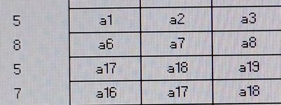
Hi, trying to find formula to divide data set in one column to 100 rows in a way that it follows sequence. Each row to divide by number of values of my choice and give me that number of columns per row. Here is presented only 3 columns. Numbers on left are my choice by how many columns by row I want to divide data set. Please check example photo.
 

Attachments

  • IMG_20230314_020912_edit_508380079417216.jpg
    IMG_20230314_020912_edit_508380079417216.jpg
    194.8 KB · Views: 10

Excel Facts

Did you know Excel offers Filter by Selection?
Add the AutoFilter icon to the Quick Access Toolbar. Select a cell containing Apple, click AutoFilter, and you will get all rows with Apple
Hi,
One way
(if i am interpreting correctly your question)
Kitap3
ABCDEFGHIJKLM
1
2DataList
3a01a02a03a04a01
4a05a06a07a08a09a02
5a10a11a12a13a14a15a16a17a03
6a18a19a20a04
7a21a05
8a22a23a24a25a06
9a26a27a07
10a28a29a30a31a32a33a34a35a36a37a08
11a38a39a40a41a42a43a44a09
12a45a46a10
13a47a48a49a50a51a52a53a54a55a11
14a56a57a58a59a60a61a62a63a12
15a64a65a66a67a13
16a68a69a70a71a72a14
17a73a74a75a76a77a78a15
18a79a80a81a82a83a84a85a16
19a86a87a88a89a90a91a92a93a94a17
20a95a96a97a98a99a100a18
21a19
22a20
23a21
24a22
25a23
26a24
27a25
28a26
29a27
30a28
31a29
32a30
33a31
34a32
35a33
36a34
37a35
38a36
39a37
40a38
41a39
42a40
43a41
44a42
45a43
46a44
47a45
48a46
49a47
50a48
51a49
52a50
53a51
54a52
55a53
56a54
57a55
58a56
59a57
60a58
61a59
62a60
63a61
64a62
65a63
66a64
67a65
68a66
69a67
70a68
71a69
72a70
73a71
74a72
75a73
76a74
77a75
78a76
79a77
80a78
81a79
82a80
83a81
84a82
85a83
86a84
87a85
88a86
89a87
90a88
91a89
92a90
93a91
94a92
95a93
96a94
97a95
98a96
99a97
100a98
101a99
102a100
Data
Cell Formulas
RangeFormula
M3:M102M3=LET(rng,B3:K20,a,IF(rng="","",rng),DROP(REDUCE(0,SEQUENCE(ROWS(a)),LAMBDA(x,y,VSTACK(x,TOCOL(FILTER(INDEX(a,y,0),INDEX(a,y,0)<>""))))),1))
Dynamic array formulas.
 
Upvote 0
Another option
Kitap3
ABCDEFGHIJKLM
1
2DataList
3a01a02a03a04a01
4a05a06a07a08a09a02
5a10a11a12a13a14a15a16a17a03
6a18a19a20a04
7a21a05
8a22a23a24a25a06
9a26a27a07
10a28a29a30a31a32a33a34a35a36a37a08
11a38a39a40a41a42a43a44a09
12a45a46a10
13a47a48a49a50a51a52a53a54a55a11
14a56a57a58a59a60a61a62a63a12
15a64a65a66a67a13
16a68a69a70a71a72a14
17a73a74a75a76a77a78a15
18a79a80a81a82a83a84a85a16
19a86a87a88a89a90a91a92a93a94a17
20a95a96a97a98a99a100a18
21a19
22a20
23a21
24a22
25a23
26a24
27a25
28a26
29a27
30a28
31a29
32a30
33a31
34a32
35a33
36a34
37a35
38a36
39a37
40a38
41a39
42a40
43a41
44a42
45a43
46a44
47a45
48a46
49a47
50a48
51a49
52a50
53a51
54a52
55a53
56a54
57a55
58a56
59a57
60a58
61a59
62a60
63a61
64a62
65a63
66a64
67a65
68a66
69a67
70a68
71a69
72a70
73a71
74a72
75a73
76a74
77a75
78a76
79a77
80a78
81a79
82a80
83a81
84a82
85a83
86a84
87a85
88a86
89a87
90a88
91a89
92a90
93a91
94a92
95a93
96a94
97a95
98a96
99a97
100a98
101a99
102a100
Data
Cell Formulas
RangeFormula
M3:M102M3=TEXTSPLIT(TEXTJOIN("|",,BYROW(B3:K20,LAMBDA(s,TEXTJOIN("|",,s)))),,"|")
Dynamic array formulas.
 
Upvote 0
If that is what the OP is trying to do, another option is
Excel Formula:
=TOCOL(B3:K20,1)
 
Upvote 0
Another option
Kitap3
ABCDEFGHIJKLM
1
2DataList
3a01a02a03a04a01
4a05a06a07a08a09a02
5a10a11a12a13a14a15a16a17a03
6a18a19a20a04
7a21a05
8a22a23a24a25a06
9a26a27a07
10a28a29a30a31a32a33a34a35a36a37a08
11a38a39a40a41a42a43a44a09
12a45a46a10
13a47a48a49a50a51a52a53a54a55a11
14a56a57a58a59a60a61a62a63a12
15a64a65a66a67a13
16a68a69a70a71a72a14
17a73a74a75a76a77a78a15
18a79a80a81a82a83a84a85a16
19a86a87a88a89a90a91a92a93a94a17
20a95a96a97a98a99a100a18
21a19
22a20
23a21
24a22
25a23
26a24
27a25
28a26
29a27
30a28
31a29
32a30
33a31
34a32
35a33
36a34
37a35
38a36
39a37
40a38
41a39
42a40
43a41
44a42
45a43
46a44
47a45
48a46
49a47
50a48
51a49
52a50
53a51
54a52
55a53
56a54
57a55
58a56
59a57
60a58
61a59
62a60
63a61
64a62
65a63
66a64
67a65
68a66
69a67
70a68
71a69
72a70
73a71
74a72
75a73
76a74
77a75
78a76
79a77
80a78
81a79
82a80
83a81
84a82
85a83
86a84
87a85
88a86
89a87
90a88
91a89
92a90
93a91
94a92
95a93
96a94
97a95
98a96
99a97
100a98
101a99
102a100
Data
Cell Formulas
RangeFormula
M3:M102M3=LET(a,TOCOL(B3:K20),FILTER(a,a<>""))
Dynamic array formulas.
 
Upvote 0
Basically that's it. However I need all values to start from same column, without blank cells, and most important I need to decide and input how many columns each row will have. I tried formula you gave me but I'm getting same info..."The first argument of Let must be a valid name".
One way
(if i am interpreting correctly your question)
Kitap3
ABCDEFGHIJKLM
1
2DataList
3a01a02a03a04a01
4a05a06a07a08a09a02
5a10a11a12a13a14a15a16a17a03
6a18a19a20a04
7a21a05
8a22a23a24a25a06
9a26a27a07
10a28a29a30a31a32a33a34a35a36a37a08
11a38a39a40a41a42a43a44a09
12a45a46a10
13a47a48a49a50a51a52a53a54a55a11
14a56a57a58a59a60a61a62a63a12
15a64a65a66a67a13
16a68a69a70a71a72a14
17a73a74a75a76a77a78a15
18a79a80a81a82a83a84a85a16
19a86a87a88a89a90a91a92a93a94a17
20a95a96a97a98a99a100a18
21a19
22a20
23a21
24a22
25a23
26a24
27a25
28a26
29a27
30a28
31a29
32a30
33a31
34a32
35a33
36a34
37a35
38a36
39a37
40a38
41a39
42a40
43a41
44a42
45a43
46a44
47a45
48a46
49a47
50a48
51a49
52a50
53a51
54a52
55a53
56a54
57a55
58a56
59a57
60a58
61a59
62a60
63a61
64a62
65a63
66a64
67a65
68a66
69a67
70a68
71a69
72a70
73a71
74a72
75a73
76a74
77a75
78a76
79a77
80a78
81a79
82a80
83a81
84a82
85a83
86a84
87a85
88a86
89a87
90a88
91a89
92a90
93a91
94a92
95a93
96a94
97a95
98a96
99a97
100a98
101a99
102a100
Data
Cell Formulas
RangeFormula
M3:M102M3=LET(rng,B3:K20,a,IF(rng="","",rng),DROP(REDUCE(0,SEQUENCE(ROWS(a)),LAMBDA(x,y,VSTACK(x,TOCOL(FILTER(INDEX(a,y,0),INDEX(a,y,0)<>""))))),1))
Dynamic array formulas.
 
Upvote 0
Can you post some sample data.

MrExcel has a tool called “XL2BB” that lets you post samples of your data that will allow us to copy/paste it to our Excel spreadsheets, so we can work with the same copy of data that you are. Instructions on using this tool can be found here: XL2BB Add-in

Note that there is also a "Test Here” forum on this board. This is a place where you can test using this tool (or any other posting techniques that you want to test) before trying to use those tools in your actual posts.
 
Upvote 0
Hi, see the linked file for a possible solution...

The formula used in the table:
=IF(AND(COLUMN()<$A2+2,SUM($A$1:$A1)+COLUMN()+2<100),INDEX(Set!$A:$A,SUM($A$1:$A1)+COLUMN()),"")

Devide.xlsx

Set.png


Devide.png
 
Upvote 0
Upvote 0
Hi, I created a new table...

The new formula used in the new table:
=IF(AND(COLUMN()<$A2+2,SUM($A$1:$A1)+COLUMN()<102),"a"&SUM($A$1:$A1)+COLUMN()-1,"")

DevideNew.xlsx

DevideNew.png
 
Upvote 0

Forum statistics

Threads
1,214,576
Messages
6,120,354
Members
448,956
Latest member
Adamsxl

We've detected that you are using an adblocker.

We have a great community of people providing Excel help here, but the hosting costs are enormous. You can help keep this site running by allowing ads on MrExcel.com.
Allow Ads at MrExcel

Which adblocker are you using?

Disable AdBlock

Follow these easy steps to disable AdBlock

1)Click on the icon in the browser’s toolbar.
2)Click on the icon in the browser’s toolbar.
2)Click on the "Pause on this site" option.
Go back

Disable AdBlock Plus

Follow these easy steps to disable AdBlock Plus

1)Click on the icon in the browser’s toolbar.
2)Click on the toggle to disable it for "mrexcel.com".
Go back

Disable uBlock Origin

Follow these easy steps to disable uBlock Origin

1)Click on the icon in the browser’s toolbar.
2)Click on the "Power" button.
3)Click on the "Refresh" button.
Go back

Disable uBlock

Follow these easy steps to disable uBlock

1)Click on the icon in the browser’s toolbar.
2)Click on the "Power" button.
3)Click on the "Refresh" button.
Go back
Back
Top