Drop-down Dynamic - List available employees

[Stefanwlb]

Hi all, I'm stumped with how to proceed. I have 11 people who list their availability for each shift for each day of the month. I made a table which has each of the employees, with days 1-30 (September) and the availability A - Available, U - Unavailable. On a separate calendar sheet, I am trying to have a dropdown list for each shift which populates only the names which have A in the cell to the right of their name, under the specific day.
any ideas

 

[KRice]

This is messy to do with older versions of Excel, but here is one approach. You will need to create helper cells that contain the names of employees who have indicated they are available for each day-shift combination. Then Data Validation is used with a formula that looks up the day and shift number on the calendar and finds the corresponding match in your helper table. I've placed everything on the same worksheet to make it easier to follow, but you can move these three major components (the input table with A's and U's, the calendar, and the helper table) wherever desired.

MrExcel_20220813.xlsx
	A	B	C	D	E	F	G	H	I	J	K	L	M	N	O	P	Q	R	S	T	U	V	W	X	Y	Z	AA	AB	AC	AD	AE	AF	AG	AH	AI	AJ
1	Date Start	9/1/2022
2
3	Day	1-Sep	1-Sep	1-Sep	2-Sep	2-Sep	2-Sep	3-Sep	3-Sep	3-Sep	4-Sep	4-Sep	4-Sep			Su	M	Tu	W	Th	F	Sa		Date	Shift	Available Staff
4	Shift -->	1	2	3	1	2	3	1	2	3	1	2	3							1	2	3		9/1/2022	1	Name1	Name2	Name5	Name6	Name8	Name9	Name11
5	Name1	A	A	U	U	A	U	A	U	A	U	A	U		1					Name6				9/1/2022	2	Name1	Name3	Name4	Name5	Name10
6	Name2	A	U	U	A	U	A	U	A	U	A	U	A		2					Name5				9/1/2022	3	Name6	Name8	Name10	Name11
7	Name3	U	A	U	U	A	U	A	U	U	A	U	U		3					Name8				9/2/2022	1	Name2	Name4	Name5	Name7	Name11
8	Name4	U	A	U	A	A	U	A	U	A	U	A	U			4	5	6	7	8	9	10		9/2/2022	2	Name1	Name3	Name4	Name7	Name8	Name9	Name10
9	Name5	A	A	U	A	U	A	A	A	A	U	A	A		1	Name6								9/2/2022	3	Name2	Name5	Name6	Name8	Name11
10	Name6	A	U	A	U	U	A	U	A	U	A	U	A		2	Name7								9/3/2022	1	Name1	Name3	Name4	Name5	Name7	Name9	Name11
11	Name7	U	U	U	A	A	U	A	U	A	U	A	U		3									9/3/2022	2	Name2	Name5	Name6	Name8	Name9	Name10
12	Name8	A	U	A	U	A	A	U	A	A	U	A	U			11	12							9/3/2022	3	Name1	Name4	Name5	Name7	Name8
13	Name9	A	U	U	U	A	U	A	A	U	A	A	U		1	Name6								9/4/2022	1	Name2	Name3	Name6	Name9	Name10	Name11
14	Name10	U	A	A	U	A	U	U	A	U	A	U	A		2									9/4/2022	2	Name1	Name4	Name5	Name7	Name8	Name9
15	Name11	A	U	A	A	U	A	A	U	U	A	U	A		3									9/4/2022	3	Name2	Name5	Name6	Name10	Name11
16																								9/5/2022	1
17																								9/5/2022	2
Stefanwlb

Cell Formulas
Range	Formula
B3:M3	B3	=DATE(YEAR($B$1),MONTH($B$1),INT((COLUMNS($B:B)-1)/3)+1)
B4:M4	B4	=MOD(COLUMNS($B:B)-1,3)+1
X4:X17	X4	=DATE(YEAR($B$1),MONTH($B$1),INT((ROWS($4:4)-1)/3)+1)
Y4:Y17	Y4	=MOD(ROWS($4:4)-1,3)+1
Z4:AJ17	Z4	=IFERROR(INDEX($A$5:$A$15,AGGREGATE(15,6,(ROW($5:$15)-ROW($5:$5)+1)/(INDEX($B$5:$M$15,,MATCH(1,($B$3:$M$3=$X4)*($B$4:$M$4=$Y4),0))="A"),COLUMNS($Z:Z))),"")

Cells with Data Validation
Cell	Allow	Criteria
P13	List	=INDEX($Z$4:$AJ$17,MATCH(1,(DAY($X$4:$X$17)=P$12)*($Y$4:$Y$17=$O13),0),)
P9:V11	List	=INDEX($Z$4:$AJ$17,MATCH(1,(DAY($X$4:$X$17)=P$8)*($Y$4:$Y$17=$O9),0),)
T5	List	=OFFSET(INDEX($Z$4:$AJ$17,MATCH(1,(DAY($X$4:$X$17)=T$4)*($Y$4:$Y$17=$O5),0),),,,,SUM(--(INDEX($Z$4:$AJ$17,MATCH(1,(DAY($X$4:$X$17)=T$4)*($Y$4:$Y$17=$O5),0),)<>"")))
U5:V7	List	=INDEX($Z$4:$AJ$17,MATCH(1,(DAY($X$4:$X$17)=U$4)*($Y$4:$Y$17=$O5),0),)
T6:T7	List	=INDEX($Z$4:$AJ$17,MATCH(1,(DAY($X$4:$X$17)=T$4)*($Y$4:$Y$17=$O6),0),)

If you have difficulty setting this up from the XL2BB mini-sheet, a copy of the worksheet is linked below. I will call your attention to the two different Data Validation formulas. The 1st one corresponding to the yellow cell uses OFFSET to dynamically adjust the length of the list of names so that no blanks are shown in the dropdown list. The other formula variant does not have this feature. As you'll see, this convenience comes at the cost of having a longer formula that requires editing in two places rather than one. About this point, because the calendar is presumed to have slots for shifts 1, 2, and 3, each of these slots needs to "look" at the day number, so the Data Validation formula needs to "fix" the row number. The problem then is that when you attempt to copy Data Validation to the next week, the formula (for DV) will require editing so that that week's formula points to the new row number where the day numbers are found. The good news is this needs to be done only one time for each week and then the week's DV formula can be copied to all days/shifts for that week.

MrExcel_20220813.xlsx

Shared with Dropbox

www.dropbox.com

 

[Stefanwlb]

Hi KRice, thank you so much for taking your time to design that. However, I am not able to grasp/understand how to apply your formula's to my own table. I have attached my sample to this post in the hopes you are able to figure it out. The columns I use are on the right of the table which is supposed to show only names that are available. The way I have set out my employee availability is by shift (each day of the month).

This is messy to do with older versions of Excel, but here is one approach. You will need to create helper cells that contain the names of employees who have indicated they are available for each day-shift combination. Then Data Validation is used with a formula that looks up the day and shift number on the calendar and finds the corresponding match in your helper table. I've placed everything on the same worksheet to make it easier to follow, but you can move these three major components (the input table with A's and U's, the calendar, and the helper table) wherever desired.

MrExcel_20220813.xlsx
	A	B	C	D	E	F	G	H	I	J	K	L	M	N	O	P	Q	R	S	T	U	V	W	X	Y	Z	AA	AB	AC	AD	AE	AF	AG	AH	AI	AJ
1	Date Start	9/1/2022
2
3	Day	1-Sep	1-Sep	1-Sep	2-Sep	2-Sep	2-Sep	3-Sep	3-Sep	3-Sep	4-Sep	4-Sep	4-Sep			Su	M	Tu	W	Th	F	Sa		Date	Shift	Available Staff
4	Shift -->	1	2	3	1	2	3	1	2	3	1	2	3							1	2	3		9/1/2022	1	Name1	Name2	Name5	Name6	Name8	Name9	Name11
5	Name1	A	A	U	U	A	U	A	U	A	U	A	U		1					Name6				9/1/2022	2	Name1	Name3	Name4	Name5	Name10
6	Name2	A	U	U	A	U	A	U	A	U	A	U	A		2					Name5				9/1/2022	3	Name6	Name8	Name10	Name11
7	Name3	U	A	U	U	A	U	A	U	U	A	U	U		3					Name8				9/2/2022	1	Name2	Name4	Name5	Name7	Name11
8	Name4	U	A	U	A	A	U	A	U	A	U	A	U			4	5	6	7	8	9	10		9/2/2022	2	Name1	Name3	Name4	Name7	Name8	Name9	Name10
9	Name5	A	A	U	A	U	A	A	A	A	U	A	A		1	Name6								9/2/2022	3	Name2	Name5	Name6	Name8	Name11
10	Name6	A	U	A	U	U	A	U	A	U	A	U	A		2	Name7								9/3/2022	1	Name1	Name3	Name4	Name5	Name7	Name9	Name11
11	Name7	U	U	U	A	A	U	A	U	A	U	A	U		3									9/3/2022	2	Name2	Name5	Name6	Name8	Name9	Name10
12	Name8	A	U	A	U	A	A	U	A	A	U	A	U			11	12							9/3/2022	3	Name1	Name4	Name5	Name7	Name8
13	Name9	A	U	U	U	A	U	A	A	U	A	A	U		1	Name6								9/4/2022	1	Name2	Name3	Name6	Name9	Name10	Name11
14	Name10	U	A	A	U	A	U	U	A	U	A	U	A		2									9/4/2022	2	Name1	Name4	Name5	Name7	Name8	Name9
15	Name11	A	U	A	A	U	A	A	U	U	A	U	A		3									9/4/2022	3	Name2	Name5	Name6	Name10	Name11
16																								9/5/2022	1
17																								9/5/2022	2
Stefanwlb

Cell Formulas
Range	Formula
B3:M3	B3	=DATE(YEAR($B$1),MONTH($B$1),INT((COLUMNS($B:B)-1)/3)+1)
B4:M4	B4	=MOD(COLUMNS($B:B)-1,3)+1
X4:X17	X4	=DATE(YEAR($B$1),MONTH($B$1),INT((ROWS($4:4)-1)/3)+1)
Y4:Y17	Y4	=MOD(ROWS($4:4)-1,3)+1
Z4:AJ17	Z4	=IFERROR(INDEX($A$5:$A$15,AGGREGATE(15,6,(ROW($5:$15)-ROW($5:$5)+1)/(INDEX($B$5:$M$15,,MATCH(1,($B$3:$M$3=$X4)*($B$4:$M$4=$Y4),0))="A"),COLUMNS($Z:Z))),"")

Cells with Data Validation
Cell	Allow	Criteria
P13	List	=INDEX($Z$4:$AJ$17,MATCH(1,(DAY($X$4:$X$17)=P$12)*($Y$4:$Y$17=$O13),0),)
P9:V11	List	=INDEX($Z$4:$AJ$17,MATCH(1,(DAY($X$4:$X$17)=P$8)*($Y$4:$Y$17=$O9),0),)
T5	List	=OFFSET(INDEX($Z$4:$AJ$17,MATCH(1,(DAY($X$4:$X$17)=T$4)*($Y$4:$Y$17=$O5),0),),,,,SUM(--(INDEX($Z$4:$AJ$17,MATCH(1,(DAY($X$4:$X$17)=T$4)*($Y$4:$Y$17=$O5),0),)<>"")))
U5:V7	List	=INDEX($Z$4:$AJ$17,MATCH(1,(DAY($X$4:$X$17)=U$4)*($Y$4:$Y$17=$O5),0),)
T6:T7	List	=INDEX($Z$4:$AJ$17,MATCH(1,(DAY($X$4:$X$17)=T$4)*($Y$4:$Y$17=$O6),0),)

If you have difficulty setting this up from the XL2BB mini-sheet, a copy of the worksheet is linked below. I will call your attention to the two different Data Validation formulas. The 1st one corresponding to the yellow cell uses OFFSET to dynamically adjust the length of the list of names so that no blanks are shown in the dropdown list. The other formula variant does not have this feature. As you'll see, this convenience comes at the cost of having a longer formula that requires editing in two places rather than one. About this point, because the calendar is presumed to have slots for shifts 1, 2, and 3, each of these slots needs to "look" at the day number, so the Data Validation formula needs to "fix" the row number. The problem then is that when you attempt to copy Data Validation to the next week, the formula (for DV) will require editing so that that week's formula points to the new row number where the day numbers are found. The good news is this needs to be done only one time for each week and then the week's DV formula can be copied to all days/shifts for that week.

MrExcel_20220813.xlsx

Shared with Dropbox

www.dropbox.com

Hi KRice, thank you so much for taking your time to design that. However, I am not able to grasp/understand how to apply your formula's to my own table. I have attached my sample to this post in the hopes you are able to figure it out. The columns I use are on the right of the table which is supposed to show only names that are available. The way I have set out my employee availability is by shift (each day of the month).

Mr excel sheet

 

[KRice]

In your source table showing names and the days of a month, I see U's and A's. But where does it show an employee's availability status for each of the three shifts on any given day? For example, Alvaro is shown as "A" (Available) for September 1, but is that "available" for First shift, Second shift, or Third shift?

 

[Stefanwlb]

In your source table showing names and the days of a month, I see U's and A's. But where does it show an employee's availability status for each of the three shifts on any given day? For example, Alvaro is shown as "A" (Available) for September 1, but is that "available" for First shift, Second shift, or Third shift?

My initial idea was to make it work for 1 shift for the entire month (i.e. list availability for Shift A for each employee, for each day of the month), and then do replicate the same thing for Shift B, etc. I see that your idea is more efficient. I have took a screenshot of the total shifts on a WEEKLY basis. Basically, Saturday/Sunday have 4 shifts available each, and Weekdays have 3 shifts.

 

[KRice]

Sorry for the delay...I was away for a week. In the example shown in post #2, I've assumed that on any given day and for any given shift, you want to be able to select just one name from the filtered list of those who have indicated their availability for that slot. Is this assumption correct?...you need only one name for the shift? I'm trying to determine if a calendar template that includes up to 4 rows for each day is sufficient, so that a name could be assigned to each of the 3 or 4 shifts for each day.

 

[KRice]

Here is a heavily revised version of your workbook that uses an approach similar to what I suggested in post #2. Enter the names in the table on the Names worksheet. Enter the beginning of month for the month to be scheduled in cell B4 of the Scheduler worksheet. Populate the body of the Scheduler table with U's and A's to indicate availability for each shift on each day. Helper columns to the right of the Scheduler table build a list of staff availability that is used next in the dropdown lists on the Calendar worksheet. About the Scheduler worksheet...the table headings (both column and row) should automatically update. This is an official Excel table, so to preserve formatting and formulas, if more staff are added to the Names table, insert another four rows in the Scheduler table (I suggest doing this between the current index 10 and 11 blocks to stay away from the bottom edge of the table)...and the formulas should handle adding the new staff member and create the shift labels. The calendar worksheet has a 6-week calendar, necessary in case a month begins on a Friday or Saturday and the last day(s) spill into the 6th week section. The month-year specified in Scheduler!B4 is carried forward to serve as a title for the calendar. Conditional formatting grays out day blocks that are not part of the month. Manual formatting grays out shift 4 for weekdays. Dropdown lists are available for each day, and selecting them refers back to the helper columns on the Scheduler worksheet where available staff are listed. A copy of the shift time blocks and locations and shift numbers is shown at right for convenient reference. Let me know if this is close to the functionality you sought.

ExampleData - MrExcel_kr.xlsx

Shared with Dropbox

www.dropbox.com

 

[Stefanwlb]

Here is a heavily revised version of your workbook that uses an approach similar to what I suggested in post #2. Enter the names in the table on the Names worksheet. Enter the beginning of month for the month to be scheduled in cell B4 of the Scheduler worksheet. Populate the body of the Scheduler table with U's and A's to indicate availability for each shift on each day. Helper columns to the right of the Scheduler table build a list of staff availability that is used next in the dropdown lists on the Calendar worksheet. About the Scheduler worksheet...the table headings (both column and row) should automatically update. This is an official Excel table, so to preserve formatting and formulas, if more staff are added to the Names table, insert another four rows in the Scheduler table (I suggest doing this between the current index 10 and 11 blocks to stay away from the bottom edge of the table)...and the formulas should handle adding the new staff member and create the shift labels. The calendar worksheet has a 6-week calendar, necessary in case a month begins on a Friday or Saturday and the last day(s) spill into the 6th week section. The month-year specified in Scheduler!B4 is carried forward to serve as a title for the calendar. Conditional formatting grays out day blocks that are not part of the month. Manual formatting grays out shift 4 for weekdays. Dropdown lists are available for each day, and selecting them refers back to the helper columns on the Scheduler worksheet where available staff are listed. A copy of the shift time blocks and locations and shift numbers is shown at right for convenient reference. Let me know if this is close to the functionality you sought.

ExampleData - MrExcel_kr.xlsx

Shared with Dropbox

www.dropbox.com

That is perfect! I was able to use that to make my scheduler much better! The only issue I see is that whenever I reopen the excel file, the dropdown menu doesn't work until I go to Data Validation - Edit - Confirm/Accept and then it works again but I have to do that for each of the dropdown lists (there is a lot of them!)
Any way to fix this?

 

[KRice]

Sorry for the delay. I don't recall encountering this behavior before, but upon opening the file, I also had the same problem. After searching quite a bit, I've concluded that many consider this to be a bug in Excel (include me in that group). I've seen posts where this issue is caused by the data validation formula exceeding a 255-character limit. That should not have been the issue here. I'm not sure why the problem is occurring. The issue has been mentioned on this forum before, for example:

Array in Data validation not saving

I have an array formula in my data validation which works fine when the workbook is open. But if I save the document, close and reopen, the validation no longer works. Its like the array is getting converted to a normal formula on open. I am working within Excel Office 365 and the file is saved...

www.mrexcel.com

...and elsewhere:

Data Validation Won't Save

I have a sub that adds data validation to a worksheet. It appears to work: Public Sub AddDataValidation(ByRef rng As Range, ParamArray options() As Variant) With rng.Validation .Delete...

stackoverflow.com

In an attempt to shorten the data validation formulas, I relied on two additional Named Ranges (created with Formulas > Name Manager). Those are for the count of staff available on any given day/shift combination (called "cntAvail"), and for an abbreviated description of the calendar day and shift number (called "codeDS"). A third Named Range ("AvailableNames") was described previously and is still used. These new ranges refer to new columns that have been added to the helper table on the Scheduler worksheet. The idea behind these new columns and Named Ranges is to shift some of the formula burden to the worksheet in-cell formulas so that the ranges containing the resulting values can be referenced with shorter names. Even with shorter data validation formulas, this did not seem to resolve the problem involving the loss of dropdown functionality, but I left these things in the revised version of the workbook.

I have yet to see an easy solution for this problem, but there is a work-around, which was borrowed from a strategy I saw here:

Redirecting

I thought using VBA to re-confirm the data validation would be straightforward, but it seems that VBA is finicky. We know the data validation formulas look at the day numbers in the calendar (to perform the lookup), but not all day number cells contain a number--some are blank and grayed out, often at the beginning of the calendar and always at the end. These blank cells with no number cause an error. If the data validation formula is entered manually, we can override the error complaint and insert the data validation formulas anyway. Not so with VBA, as discussed here:

How to add erroneous list-formula validation in VBA?

In the Excel UI you can enter a list-type validation whose list is a formula that results in an error. If you do, a dialog box comes up saying "The Source currently evaluates to an error. Do you want to continue?", and if you say Yes, it will preserve the validation. For example, the Source...

www.mrexcel.com

So, borrowing another idea from this post, the VBA code is extended to first overwrite the day number formula in all of the cells with 1's. The number 1 everywhere is seen as a valid "day" number, so the VBA code can successfully re-insert the data validation formulas without terminating due to an error. Then we overwrite the 1's with the day-numbering formula to restore the correct day numbers.

There is very likely a more efficient way to code this, but this worked for me...the "resetDV" code refers to the internal worksheet name assigned to the latest version of the calendar sheet (CalV2 internally, sheet called "Calendar_v2", but can be renamed as desired):

Sub resetDV()
'
' Kirk Rice 9/21/2022
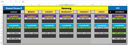
' resetDV Macro is run to automatically reset Data Validation to enable dropdown selection of staff available for a specified shift and day
' Uses three Named Ranges in the Excel workbook
'
    Dim AvailableNames, codeDS, cntAvail
'
' Overwrite top cells for each day with "1", a valid day everywhere...to prevent terminaton of code execution when an invalid blank "day" number is encounterd.
'
    CalV2.Range("B4:H4,B9:H9,B14:H14,B19:H19,B24:H24,B29:H29").Value = 1
'
' Re-enter Data Validation formulas to re-activate dropdown selection
    With CalV2.Range("B5:H8").Validation
        .Delete
        .Add Type:=xlValidateList, AlertStyle:=xlValidAlertStop, Operator:= _
         xlBetween, Formula1:="=OFFSET(INDEX(AvailableNames,MATCH(1,--(codeDS=B$4&""-""&$A5),0),),,,,INDEX(cntAvail,MATCH(1,--(codeDS=B$4&""-""&$A5),0)))"
        .IgnoreBlank = True
        .InCellDropdown = True
        .InputTitle = ""
        .ErrorTitle = ""
        .InputMessage = ""
        .ErrorMessage = ""
        .ShowInput = True
        .ShowError = True
    End With
    With CalV2.Range("B10:H13").Validation
        .Delete
        .Add Type:=xlValidateList, AlertStyle:=xlValidAlertStop, Operator:= _
        xlBetween, Formula1:="=OFFSET(INDEX(AvailableNames,MATCH(1,--(codeDS=B$9&""-""&$A10),0),),,,,INDEX(cntAvail,MATCH(1,--(codeDS=B$9&""-""&$A10),0)))"
        .IgnoreBlank = True
        .InCellDropdown = True
        .InputTitle = ""
        .ErrorTitle = ""
        .InputMessage = ""
        .ErrorMessage = ""
        .ShowInput = True
        .ShowError = True
    End With
    With CalV2.Range("B15:H18").Validation
        .Delete
        .Add Type:=xlValidateList, AlertStyle:=xlValidAlertStop, Operator:= _
        xlBetween, Formula1:="=OFFSET(INDEX(AvailableNames,MATCH(1,--(codeDS=B$14&""-""&$A15),0),),,,,INDEX(cntAvail,MATCH(1,--(codeDS=B$14&""-""&$A15),0)))"
        .IgnoreBlank = True
        .InCellDropdown = True
        .InputTitle = ""
        .ErrorTitle = ""
        .InputMessage = ""
        .ErrorMessage = ""
        .ShowInput = True
        .ShowError = True
    End With
    With CalV2.Range("B20:H23").Validation
        .Delete
        .Add Type:=xlValidateList, AlertStyle:=xlValidAlertStop, Operator:= _
        xlBetween, Formula1:="=OFFSET(INDEX(AvailableNames,MATCH(1,--(codeDS=B$19&""-""&$A20),0),),,,,INDEX(cntAvail,MATCH(1,--(codeDS=B$19&""-""&$A20),0)))"
        .IgnoreBlank = True
        .InCellDropdown = True
        .InputTitle = ""
        .ErrorTitle = ""
        .InputMessage = ""
        .ErrorMessage = ""
        .ShowInput = True
        .ShowError = True
    End With
    With CalV2.Range("B25:H28").Validation
        .Delete
        .Add Type:=xlValidateList, AlertStyle:=xlValidAlertStop, Operator:= _
        xlBetween, Formula1:="=OFFSET(INDEX(AvailableNames,MATCH(1,--(codeDS=B$24&""-""&$A25),0),),,,,INDEX(cntAvail,MATCH(1,--(codeDS=B$24&""-""&$A25),0)))"
        .IgnoreBlank = True
        .InCellDropdown = True
        .InputTitle = ""
        .ErrorTitle = ""
        .InputMessage = ""
        .ErrorMessage = ""
        .ShowInput = True
        .ShowError = True
    End With
    With CalV2.Range("B30:H33").Validation
        .Delete
        .Add Type:=xlValidateList, AlertStyle:=xlValidAlertStop, Operator:= _
        xlBetween, Formula1:="=OFFSET(INDEX(AvailableNames,MATCH(1,--(codeDS=B$29&""-""&$A30),0),),,,,INDEX(cntAvail,MATCH(1,--(codeDS=B$29&""-""&$A30),0)))"
        .IgnoreBlank = True
        .InCellDropdown = True
        .InputTitle = ""
        .ErrorTitle = ""
        .InputMessage = ""
        .ErrorMessage = ""
        .ShowInput = True
        .ShowError = True
    End With
    Range("A1").Select
'
' Overwrite temporary "valid" 1's with formula to display the correct day numbers aligned under the days of the week headings
'
    CalV2.Range("B4:H4,B9:H9,B14:H14,B19:H19,B24:H24,B29:H29").Formula = _
    "=IF(OR(7*INT((ROWS($4:4)-1)/5)+COLUMNS($B:B)-WEEKDAY($B$1)+1>DAY(EOMONTH($B$1,0)),7*INT((ROWS($4:4)-1)/5)+COLUMNS($B:B)-WEEKDAY($B$1)+1<1),"""",7*INT((ROWS($4:4)-1)/5)+COLUMNS($B:B)-WEEKDAY($B$1)+1)"
'
End Sub

This macro is placed inside an Auto Open routine so that when the file is opened, it automatically runs to re-confirm the data validation cells to restore normal operation.

Due to space limitations, only the upper left of the helper table on the Scheduler sheet is shown, to provide some idea about how it works:

ExampleData - MrExcel_kr.xlsm
	AO	AP	AQ	AR	AS	AT
7	Date	Shift	codeDS	cntAvail	Available Staff
8	12/1/2022	1	1-1	2	Alvaro	Shea
9	12/1/2022	2	1-2	1	Sam
10	12/1/2022	3	1-3	1	Liam
Scheduler

Cell Formulas
Range	Formula
AO8:AO10	AO8	=IF(ROWS($6:6)<=COUNT($D$6:$AH$6)*4,DATE(YEAR($B$4),MONTH($B$4),INT((ROWS($6:6)-1)/4)+1),"")
AP8:AP10	AP8	=IF(ROWS($6:6)<=COUNT($D$6:$AH$6)*4,MOD(ROWS($6:6)-1,4)+1,"")
AQ8:AQ10	AQ8	=DAY(AO8)&"-"&AP8
AR8:AR10	AR8	=SUMPRODUCT(--(AS8:BC8<>""))
AS8:AT10	AS8	=IFERROR(INDEX(Table3[[Employee Name]:[Employee Name]],AGGREGATE(15,6,(ROW(Table3[[Employee Name]:[Employee Name]])-ROW($8:$8)+1)/((INDEX(Table3[[Col1]:[Col31]],,MATCH(1,--($D$6:$AH$6=DAY($AO8)),0))="A")*(Table3[[Shift]:[Shift]]=$AP8)),COLUMNS($AS:AS))),"")

Named Ranges
Name	Refers To	Cells
AvailableNames	=Scheduler!$AS$8:$BC$131	AO10:AP10, AR8, AS8:AT10
cntAvail	=Scheduler!$AR$8:$AR$131	AO10:AP10, AS8:AT10
codeDS	=Scheduler!$AQ$8:$AQ$131	AO10:AP10, AS8:AT10
Dates	=Scheduler!$AO$8:$AO$131	AO10:AP10, AS8:AT10, AQ8
Shifts	=Scheduler!$AP$8:$AP$131	AO10:AP10, AS8:AT10, AQ8

I've uploaded the revised version of this workbook, available here:

ExampleData - MrExcel_kr.xlsm

Shared with Dropbox

www.dropbox.com

Note that this version is set to run the macro upon opening, so you may need to adjust security settings to allow for that. If you want to open the file without running the VBA, hold down the shift key while using File > Open and clicking on the file name.