Drop Down Lists with Criteria

[MrUnsurewhattodo]

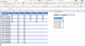
Hi all, im trying to add in a drop down list with criteria.

We have products and builders and I would like to be able to select which builder for individual products based on those that can build it (not all builders and build all products). So I would like to select a product and then only the builders that can build up show in the drop down box J3

Ive added a example file and already have the dropdown for the product I3

Please help

 

[Toadstool]

Hi MrUnsurewhattodo,

There may be a forum member along soon who can provide a solution better suited to your Excel 365 version but as I've only Excel 2016 then this is my approach.

For the Builder selection you'll need to construct the Data Validation List of each Builder with a "YES" against that Product. I'm guessing that you may want to copy down the selection cells so the list will need to be built horizontally, one for each Product selection cell.

Here I've used columns M to R but they could be hidden or further off to one side. The selection would look like this:

Here would be the formulae

Unsurewhattodo.xlsx
	A	B	C	D	E	F	G	H	I	J	K	L	M	N	O	P	Q	R
1	Product Code	Callum	Colin	Luke	Chris	Andy	Kiann
2	ACC1948	YES	YES	YES			YES		Product	Builder
3	ACC1192	YES	YES			YES			ACC1470	Andy			Callum	Colin	Andy
4	ACC1470	YES	YES			YES			ACC1303	Colin			Colin	Chris
5	ACC1801		YES	YES					ACC1255	Chris			Colin	Chris
6	ACC1303		YES		YES				ACC1635	Kiann			Callum	Colin	Luke	Chris	Andy	Kiann
7	ACC1255		YES		YES				ACC1750				Colin	Luke	Andy
8	ACC1820		YES		YES
9	ACC1827		YES
10	ACC1750		YES	YES		YES
11	ACC1310		YES
12	ACC1487		YES
13	ACC1253		YES
14	ACC1618		YES
15	ACC1565		YES
16	ACC1635	YES	YES	YES	YES	YES	YES
17
Sheet1

Cell Formulas
Range	Formula
M3:R13	M3	=IFERROR(INDEX(Table1[[#Headers],[Callum]:[Kiann]],AGGREGATE(15,6,COLUMN(Table1[[#Headers],[Callum]:[Kiann]])-COLUMN(Table1[[#Headers],[Product Code]])/(INDEX(Table1[[Callum]:[Kiann]],MATCH($I3,Table1[Product Code],0),)="YES"),COLUMN()-COLUMN($L$3))),"")

Cells with Data Validation
Cell	Allow	Criteria
I3:I16	List	=$A$2:$A$16
J3:J16	List	=OFFSET($M3,,,,COUNTIF($M3:$R3,"> "))