Drop Down menu based on the month

[JamieLee2k]

I will try to explain this the best way I can.
So there is a game called Animal Crossing and in the game you can catch Bugs and Fish, I am looking to make an excel sheet where I can choose from a drop down menu for a certain month so only the relavent fish or bugs show up so I know what is available for my specific month.

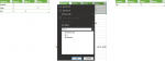
Lets narrow this down and give you an example of how it would look

Above are examples of how it will be layed out but what I need to do is add multiple months to each bug and then I can filter them to only display based on the month I select, a common Bluebottle is available from April-August and a Paper Kite Butterfly is available from Jan-Dec and a greate purple emperor from May-August, Since there are multiple months for each bug I want a drop down so say I select April it will only select bugs for april, I can do the drop down menu what I can't do is create multiple months and only select them

 

[C Moore]

You didn't mention what version Excel you're running. 365 has a new function that would let you enter in this one formula:
=FILTER(animals,INDEX(tableofchecks,,MATCH(dropdown,monthheaders)="✓")

 

[JamieLee2k]

I am running 2013 version

 

[C Moore]

If you format as a table, you can click the filter arrow and select the check. In attached example filtered for April.

 

[Dossfm0q]

Greetings JamieLee2k and All

I think you Need to use "INDEX" Function, If so Please Name cells Range below Month with Name to Use "INDIRECT" function
and to be copy and Paste Function if your Table similar to Below Table then Press Ctrl +Shift + Enter or it will not works, to be Between { }
"=IFERROR(INDEX($A$2:$P$5;SMALL(IF(INDIRECT($A$7)=$B$7;ROW($A$2:$A$5)-1;"");ROW(A1));1);"")"

and this to Save Time for Name Range Titled with Months Name

Sub To_Name_Ranges()

For Each Rng In ActiveSheet.Range("E1:P1")
ActiveWorkbook.Names.Add Name:=Rng.Value, RefersTo:="=" & Rng.Offset(1, 0).Resize(4, 1).Address

Next
End Sub

=IFERROR(INDEX($A$2:$P$5;SMALL(IF(INDIRECT($A$7)=$B$7;ROW($A$2:$A$5)-1;"");ROW(A1));1);"")

 

[Dossfm0q]

Here I Used XLBB the Last Right Button

match.xlsm
	A	B	C	D	E	F	G	H	I	J	K	L	M	N	O	P
1	Bugs				Jan	Feb	Mar	Apr	May	Jun	Jul	Aug	Sep	Oct	Nov	Dec
2	Common bluebottle	300	Flying	4 AM - 7 PM	-	-	-	✓	✓	✓	✓	✓	-	-	-	-
3	Paper kite butterfly	1,000	Flying	8 AM - 7 PM	✓	✓	✓	✓	✓	✓	✓	✓	✓	✓	✓	✓
4	Great purple emperor	3,000	Flying	4 AM - 7 PM	-	-	-	-	✓	✓	✓	✓	-	-	-	-
5	Monarch butterfly	140	Flying	4 AM - 5 PM	✓	✓	✓	✓	✓	✓	✓	✓	✓	✓	✓	✓
6
7	Jan	✓
8	Paper kite butterfly
9	Monarch butterfly
10
11
4

Cell Formulas
Range	Formula
A8:A11	A8	=IFERROR(INDEX($A$2:$P$5,SMALL(IF(INDIRECT($A$7)=$B$7,ROW($A$2:$A$5)-1,""),ROW(A1)),1),"")
Press CTRL+SHIFT+ENTER to enter array formulas.

Named Ranges
Name	Refers To	Cells
Apr	='4'!$H$2:$H$5	A8:A11
Aug	='4'!$L$2:$L$5	A8:A11
Dec	='4'!$P$2:$P$5	A8:A11
Feb	='4'!$F$2:$F$5	A8:A11
Jan	='4'!$E$2:$E$5	A8:A11
Jul	='4'!$K$2:$K$5	A8:A11
Jun	='4'!$J$2:$J$5	A8:A11
Mar	='4'!$G$2:$G$5	A8:A11
May	='4'!$I$2:$I$5	A8:A11
Nov	='4'!$O$2:$O$5	A8:A11
Oct	='4'!$N$2:$N$5	A8:A11
Sep	='4'!$M$2:$M$5	A8:A11

Cells with Data Validation
Cell	Allow	Criteria
A7	List	=$E$1:$P$1

 

[Fluff]

I am running 2013 version

Can you please update your account details to show this, as it affects which functions you can use. Thanks

Another option, without volatile functions, or named ranges.

+Fluff New.xlsm
	A	B	C	D	E	F	G	H	I	J	K	L	M	N	O	P
1	Bugs				Jan	Feb	Mar	Apr	May	Jun	Jul	Aug	Sep	Oct	Nov	Dec
2	Common bluebottle	300	Flying	4 AM - 7 PM	-	-	-	✓	✓	✓	✓	✓	✓	-	-	-
3	Paper kite butterfly	1000	Flying	8 AM - 7 PM	✓	✓	✓	✓	✓	✓	✓	✓	-	✓	✓	✓
4	Great purple emperor	3000	Flying	4 AM - 7 PM	-	-	-	-	✓	✓	✓	✓	-	-	-	-
5	Monarch butterfly	140	Flying	4 AM - 5 PM	✓	✓	✓	✓	✓	✓	✓	✓	✓	✓	✓	✓
6
7	Apr	✓
8	Common bluebottle
9	Paper kite butterfly
10	Monarch butterfly
Sheet1

Cell Formulas
Range	Formula
A8:A10	A8	=IFERROR(INDEX($A$2:$A$5,AGGREGATE(15,6,(ROW($A$2:$A$5)-ROW($A$2)+1)/($E$1:$P$1=$A$7)/($E$2:$P$5=$B$7),ROWS(A$8:A8))),"")