Dynamic Data Validation List

[Bkisley]

Hello experts!
I have a form my users will fill out. On this form there will be two columns that will require drop downs.
Right now I have the inefficient way of having two completely separate lists when in reality what I need is to have my 2nd drop down dynamic based on the 1st column drop down

On my "Welcome" tab - Cells A50:A100 is my "Main Category" header/values and cells B50:B100 is my "Subcategory" header/values
The user will fill out this welcome tab initially to set up their own personalized document.
Example: The user could type in "Painting" in cell A51 "Plumbing" in cell A52 and "Interior" in B51 and and "Residential" in B52

What I need is for my 2nd drop down to be based on what is chosen in my first drop down SO if the user selects "Painting" in my first drop down the only option based in the above example that would show up is "Interior". The option for "residential should not show up!. The reverse is true if the user selects "Plumbing" only "Residential" should should

Currently my drop downs are pulling from a pivot table that was created so I only have unique values for my Main Category values and a separate pivot table for my Sub category values. Obviously the issue that has is my 2nd drop down could have 50 options that really are not options that are paired with my first drop down selection.

My range of categories has to be dynamic - currently in a table to do this.
There has to be an efficienty way to do this!

 

[maabadi]

1. Use Name Manager for Define Name for Both List (Main Category (Headers) & Each Element of it (Sub Headers) ) For Example
* Main Category is Country Name With Name of Countries ( For Example : B1:D1 )
* For Each Country Name (For Example USA, UK, Germany, ...) , Name Manger Name is Exactly Name of Element at Main Category and Then Select Range for Sub headers ( Here Cities for Each Country , For Example : B2:B8 for First Country, C2:C10 for Second Country & D2:D7 for 3rd Country)
2. Select Range for Main List (For Example F1). Go to Data Validation Select List and Enter
= Main Category Name (What you named, Here Countries)
3. Select Range for Main List, But at Source write =INDIRECT(F1)
INDIRECT(your main list address)
4. Now It is Ready. when select from main list, sub list is updated.

 

[Bkisley]

Hello, what I am trying to do here is create a template that many people will be using and their list will be fully customized and unique. The example you did above makes perfect sense and it works, however that is a fixed set of data. What I will have is a completely unique set of data for each user that can constantly change.

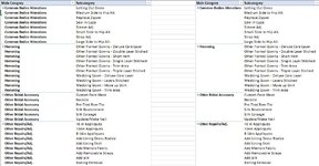
I have attached a screen shot of a pivot table that has examples of the complexity I am dealing with for one of my potential users. These are two identical sets of pivot tables except the right doesn't repeat labels. Only need one to show unique scenarios, however I thought seeing both versions wouldn't hurt. The pivot tables are pulling from data table I have on my Welcome tab as noted in my first post.

I need to be able to select the main category in my first drop down and select Common Bodice Alterations, Hemming, Other Bridal Accessory, or Other Repairs/adj
Based on that selection, my next drop down needs to only show what are the sub categories that go with the main category

In my attached example --> Other Bridal Accessory in the first drop down and the 2nd drop down I would only be able to see and select custom face mask, necktie, pre-tied bow tie, silk boutonniere, silk corsage, update/make veil. nothing else should be shown in this second drop down.

I can use what you said above sure, but that only works after the fact. After I already have all this data in here. I could have one main category or 30 for example. It needs to be built so it is ready for whatever the user throws at it.

 

[maabadi]

1. Please Update your Account details to we know what version of Excel you Use.
2. If you do above process correctly, when you select main category at first dropdown, Second dropdown only show the items have under main category at source named range.

 

[Bkisley]

I get that. My issue is that process works if AND ONLY IF you know what each main category header is. If I add in a new main category then your process requires that the user would have to follow your process each time. I can't have that. The items that will show up in the drop down come from a table. When the user gets their file, it will be a blank table that they fill out. This means they would have to do this. I am trying to find a way to have this automatically done aka dynamic.

 

[maabadi]

You Can Use Second way:
1. Select All range You want As Main Headers (for now and next). Go to Define Name & Give it name (e.g. MainList)
2. Select All Range you want to Main Headers and Sub Headers. For Example B1:CZ30 . (more Than 100 column)
3. Go to Create From Selection and then Select only top row, you can see all of them added to Name manager.
4. Select the cell you want first dropdown (e.g. A1 ). Go to Data Validation and Select list and =MainList
5. Select the cell you want second dropdown (e.g. A2 ). Go to Data Validation and Select list and =INDIRECT(A1&"_")

 

[Bkisley]

This does not work. I have tried it multiple times to no success. Whenever I do the second drop down after I click ok after typing in =INDIRECT(M10&"_") (M10 is the location of my first drop down in the example I just tried) I get the following box "The Source currently evaluates to an error. Do you want to continue?" I click yes and then the second drop down does nothing. What am I missing?

 

[Akuini]

Hi, Bkisley

1. Indirect won't work with dynamic named range.
2. Could you upload a sample workbook to a free site such as dropbox.com or google drive & then put the link here? It will make it easier to test and find a solution.
3. If you're interested, I have an example of multiple dependent data validation with dynamic range, but it uses VBA not formula.

 

[Bkisley]

Book2.xlsx

drive.google.com

That is a link to an example.
If the VBA doesn't slow my full file down I would be interested. The full file is quite large and has several codes already in it that do a lot of things for me. I won't rule it out! Thank you guys for sticking with me!

 

[Akuini]

Ok, try this:

data validation list - Bkisley - 1.xlsm

Shared with Dropbox

www.dropbox.com

the instruction on how to set it up is in this example:

dhee - 3 data validation, unique, dependent, dynamic row, relative column.xlsm

Shared with Dropbox

www.dropbox.com

In short, what you should do are:
Create a named range “xName”, refers to a cell, any cell will do.
In the data validation (in both column) use source: =xName
You need a helper column in the data/source sheet

In sheet1 code module: adjust the code in this part:
'=============== YOU MAY NEED TO ADJUST THE CODE IN THIS PART:

If the VBA doesn't slow my full file down I would be interested.

Most of the process will be done in memory not in the sheet, so I don't think it will be slow. But you need to try it on your large data.