Dynamic INDEX/MATCH-function with 2 value-identities

[deadlyjack]

The names of the products on the picture is NOT our products. I've made a look alike theme, with made up names, picturing the question I'd like help with.

I need to purchase tons of flavours/month in order to keep production afloat, amongst many other products.

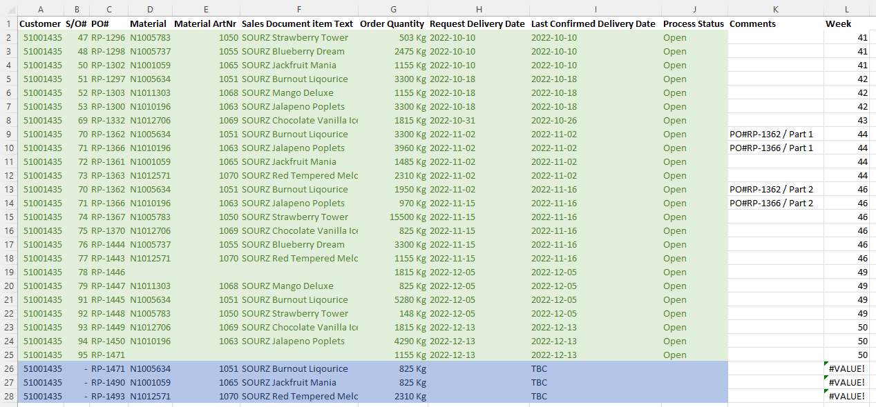
The flavours are a big aspect to the planning. If you examine, pic 2, you'll see that there are many rows with the same material ArtNr. These all have different approved delivery dates. To make it easier on my behalf, I also added, Week, in column L, just so that I can sort out which week number the different orders will arrive, =ISOWEEKNUM(I2).

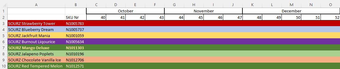
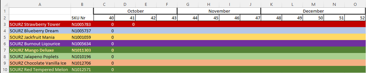
pic 1 displays an empty Forecast that I'd like to automate the Order Quantity (Column G in pic 2)

If I try this formula in sheet, Powder, on D3, I'll get the results perfect:

=IFERROR(INDEX('Orders'!$D:$G;SMALL(IF('Orders'!$D:$D=Powder!$B$3;ROW('Orders'!$L:L));ROW(1:1));4);"")
Result: 503 for week 41

But How do I make this dynamic (to the right), where the formula detects both the SKU Nr & Weeknr (Column D & L in sheet, Orders) between C3:O10 in sheet, Powder? I guess that I would need to convert the weeknumbers row in pic 2, to find the right cell for the weeknumbers column in pic 1

I need the kilo amount for each weeknr in order to plan production ahead of time.

pic 1 (Sheetname = Powder)

pic 2 (Sheetname = Orders)

We've been adding the numbers manually & I really would like this particular issue to work by itself

 

[arc6th]

In Powder!C3: =SUMIFS(Orders!G:G,Orders!D:D,$B3,Orders!L:L,C$2) Drag it down and to the right.

It should work assuming the Order Quantity column are actually numbers with 'Kg' added via formatting. If the Order Quantity column is full of text that's tough to sum.

 

[deadlyjack]

When I try your suggestion, I get the result back as 0 & it doesn't seem to be a dynamic solution,. According to the sheet kg is cell formatted:

My current solution is based on a dynamic idea for dragging downwards, see example, selected cell is D3 while draged down the formula:

the numbers in D4 & D5 is the rest of the values for N1005783, Row 3, but the weeknumbers with blank value doesn't add between each week + I need the numbers to be added to the right, not downwards... That's why I was hoping one could combined SKU Nr & weeknumber to find it's right position in my forecasting-table.

 

[arc6th]

Oops. I failed to lock the column references to the Orders tab. Enter the formula into C2:

C2: =SUMIFS(Orders!$G:$G,Orders!$D:$D,$B3,Orders!$L:$L,C$2

Drag it to the right to Week 41, and then drag it down in just that column as a test.

 

[deadlyjack]

Hmm... I receive zeros, could be the KG in the cells... Ionno...
Selected cell is D3.

But I'll try to use this formula the best I can!
Thanks!

 

[deadlyjack]

Thanks it worked nicely!
I just added a bit of coding, since I don't want the 0's to pop up everywhere:

=IF(SUMIFS(Orders!$G:$G,Orders!$D:$D,$B3,Orders!$L:$L,C$2);SUMIFS(Orders!$G:$G,Orders!$D:$D,$B3,Orders!$L:$L,C$2);"")

Changed columns accordingly within the formula, so all of the weekly schedule is in order

Thanks for the help!

 

[Peter_SSs]

I just added a bit of coding, since I don't want the 0's to pop up everywhere:

=IF(SUMIFS(Orders!$G:$G,Orders!$D:$D,$B3,Orders!$L:$L,C$2);SUMIFS(Orders!$G:$G,Orders!$D:$D,$B3,Orders!$L:$L,C$2);"")

If you are using your 365 version then you can do that more efficiently like this (with ; separators instead of commas?)
It is not only shorter, but also saves Excel doing the same calculation twice if not zero.

=LET(s,SUMIFS(Orders!$G:$G,Orders!$D:$D,$B3,Orders!$L:$L,C$2),IF(s,s,""))

 

[deadlyjack]

Amazing! This is exactly what I wanted & it works perfectly!
Since my workbook will be loaded with major tasks, I need the algorithm that requires the least memory access (mems).

Yeah, I need the ; instead of the commas but is easy to change!

 

[Peter_SSs]

Glad to help. Thanks for the follow-up.