mholland1187
New Member
- Joined
- Mar 10, 2021
- Messages
- 2
- Office Version
- 2016
- Platform
- Windows
I have searched through google for about five and a half hours trying to find a formula for this with no luck.
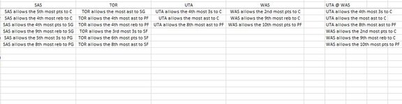
I am trying to create a dynamic list that could possibly be part of an either/or function. I have columns of all 30 NBA teams and all their rankings against each opposition position for each statistic. Basically what I would like to do is create one dynamic list that shows me all of the notes below the team name. For example, if UTA were to play WAS, I would like to have all 3 notes from the UTA column and all 3 notes from the WAS column be combined into one dynamic list of 6 on another tab. I understand I can do this by copy and paste, but I would prefer a formula if possible. I've found instruction if the columns are side by side (obviously the team names will not always be as they are alphabetical), but that would require a lot of manual cut and paste and again, I would like to eliminate as much manual work as possible. The range is 600 cells (30 columns x 20 rows) if that matters with the team abbreviations across the header row. The notes below are dynamic from another part of the spreadsheet, but will not go past 20 rows.
A couple starter ideas I had, but could not create formulas for
If the 3 left cells = UTA or WAS, then dynamic list combined
Match column title UTA and WAS, then dynamic list combined
I attached a snippet of the end of the data with the ideal output 6 lines from both teams. The header for that can be built into the formula or not, it doesn't matter.
If anyone could help, it would be greatly appreciated. I can provide any additional information if necessary. The hardest part I've found when searching for help or how to in excel is finding the correct terminology or not explaining myself fully so please bear with me!
")


