Dynamic Range, with Indirect?

[randyharris]

Can't figure this one out.

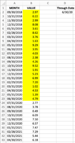
A1 that has a starting end of month date
A2 has an ending start of month date

Column B has a long list of end of month dates

Columns C through N have data in them related to the month end dates

I'm trying to use the value in cells A1 and A2 to dynamically adjust my formulas that look at the data in columns C through N, I'd like to be able to adjust those dates in A1 and A2 and have the formula adjust to the starting and ending rows which equal those dates. I've tried looking for INDIRECT and OFFSET to get the results, but can't get it right.

 

[Eric W]

It really depends on what your formulas are. Here's one possibility:

Book2
	A	B	C	D	E
1	1/31/2020	Date
2	10/31/2020	1/31/2019		A	1
3		2/28/2019		B	2
4		3/31/2019		C	3
5	Sum	4/30/2019		D	4
6	175	5/31/2019		E	5
7		6/30/2019		F	6
8		7/31/2019		G	7
9		8/31/2019		H	8
10		9/30/2019		I	9
11		10/31/2019		J	10
12		11/30/2019		K	11
13		12/31/2019		L	12
14		1/31/2020		M	13
15		2/29/2020		N	14
16		3/31/2020		O	15
17		4/30/2020		P	16
18		5/31/2020		Q	17
19		6/30/2020		R	18
20		7/31/2020		S	19
21		8/31/2020		T	20
22		9/30/2020		U	21
23		10/31/2020		V	22
24		11/30/2020		W	23
25		12/31/2020		X	24
26		1/31/2021		Y	25
27		2/28/2021		Z	26
28		3/31/2021		AA	27
29		4/30/2021		AB	28
30		5/31/2021		AC	29
Sheet3

Cell Formulas
Range	Formula
A6	A6	=SUM(INDEX(E:E,MATCH(A1,B1:B30,0)):INDEX(E:E,MATCH(A2,B1:B30,0)))

 

[joeu2004]

Here's one possibility:
[....]
=SUM(INDEX(E:E,MATCH(A1,B1:B30,0)):INDEX(E:E,MATCH(A2,B1:B30,0)))

Or simply:

=SUMIFS(E1:E30, B1:B30, ">=" & A1, B1:B30, "<=" & A2)

PS.... Well, I only looked at Eric's example. Upon reading the OP, I think Eric's example was just over-simplified. Assuming values in columns E:G:

=SUM(INDEX(E1:E30,MATCH(A1,B1:B30,0)):INDEX(G1:G30,MATCH(A2,B1:B30,0)))

 

[joeu2004]

I've tried looking for INDIRECT and OFFSET to get the results

As Eric wrote: it depends on your formulas and, in particular, whether you need to iterate over all of the data in C:N in one formula, or your intent is to have separate formulas for each column.

The take-away is: avoid using INDIRECT and OFFSET. They are "volatile" functions. That means: any formulas that use them and formulas that refer directly or indirectly to formulas that use them are recalculated every time Excel decides to recalculate anywhere in the workbook. For example, editing. But there are operations that cause recalculations.

If you only have a few such formulas, no problem. But when you have 100s or 1000s, things get really slow. Ever see complaints from users about Excel becoming "non-responsive", or opening or saving files takes "minutes". 99 times out of 100, it is the use of "volatile" functions, especially with whole-column ranges like C:C.

Bottom line: the more specific you are in your question, with complete and concrete examples that are representative of the data and formulas, the better ours answers will be.

 

[randyharris]

As Eric wrote: it depends on your formulas and, in particular, whether you need to iterate over all of the data in C:N in one formula, or your intent is to have separate formulas for each column.

The take-away is: avoid using INDIRECT and OFFSET. They are "volatile" functions. That means: any formulas that use them and formulas that refer directly or indirectly to formulas that use them are recalculated every time Excel decides to recalculate anywhere in the workbook. For example, editing. But there are operations that cause recalculations.

If you only have a few such formulas, no problem. But when you have 100s or 1000s, things get really slow. Ever see complaints from users about Excel becoming "non-responsive", or opening or saving files takes "minutes". 99 times out of 100, it is the use of "volatile" functions, especially with whole-column ranges like C:C.

Bottom line: the more specific you are in your question, with complete and concrete examples that are representative of the data and formulas, the better ours answers will be.

Index Match situation won't work as that brings a single number. I'm trying to attach an image to show it better. My FROM date is know, in this example it's always A2, and my starting sum value is B2. Based on the Through Date in D2, I need a formula that has a dynamic range from B2 through the row in column B which coinsides with the Through Date, in this example row 23.

 

[randyharris]

Oohhhh, I did try those index match sum formulas and they work fabulously - thanks everybody.

 

[Eric W]

I have a few thoughts. If your start cell is always B2, you can use this formula (based on your example in post 5):

=SUM(B2:INDEX(B:B,MATCH(D2,A1:A30,0)))

Second, as joeu2004 pointed out, this is an ideal situation for SUMIFS (or even SUMIF if your version of Excel doesn't have SUMIFS):

=SUMIF(A:A,"<="&D2,B:B)


In any case, I'm glad you got it working, and that we could help!

 

[randyharris]

I have a few thoughts. If your start cell is always B2, you can use this formula (based on your example in post 5):

=SUM(B2:INDEX(B:B,MATCH(D2,A1:A30,0)))

Second, as joeu2004 pointed out, this is an ideal situation for SUMIFS (or even SUMIF if your version of Excel doesn't have SUMIFS):

=SUMIF(A:A,"<="&D2,B:B)


In any case, I'm glad you got it working, and that we could help!

I’ve implemented the solution just as you showed here with the B2:INDEX solution.

not sure I’ll change it mow to the SUMIF solution, that is clean and simple, off hand I’m unsure if Mac Excel 2019 has SUMIFS or not but how would the SUMIFS implementation work better than the SUMIF formula shown?

 

[Eric W]

The SUMIFS would be required if your data didn't always start at B2. You'd need 2 conditions, one for the upper bound as SUMIF has, and another for the lower bound. It would also work if your data wasn't sorted.

The formula you used is pretty clean and simple, and if you understand it, and it works for you, I see no reason to try something else. Best wishes!