Dynamic Range

ldoodle

New Member
Joined
Mar 2, 2010
Messages
37
Hey,

I need to create a dynamic range so it ignores blanks. I've used the OFFSET feature in the past to achieve this, but this time my blanks are actually formulas returning nothing (""). This doesn't seem to be seen as blank!

I've seen this thread http://www.mrexcel.com/forum/excel-...ge-ignoring-formulas-result-empty-output.html but it doesn't help.

'Blank' Cell formula:
Code:
=IF(ISBLANK(_ExtData!C8),"",_ExtData!C8)

DR Refers to:
Code:
=_Data!$B$2:$H$14:INDEX(_Data!$B2:$B14,MATCH(1,1/(Data!$B$2:$B$14=""),0)-1)

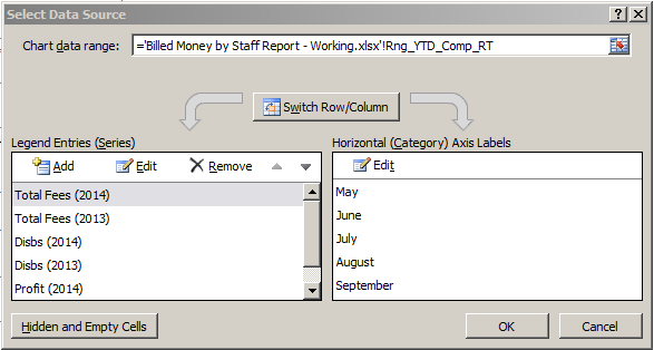
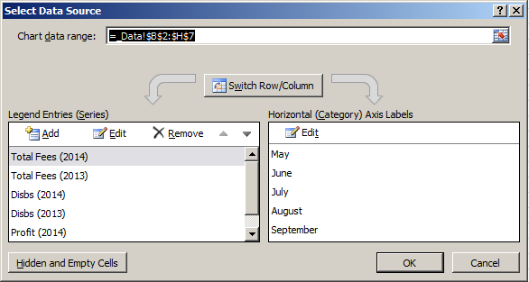
What am I doing wrong? Basically I need to select multiple columns until we reach a 'blank' row, for use by a Chart.

Thanks

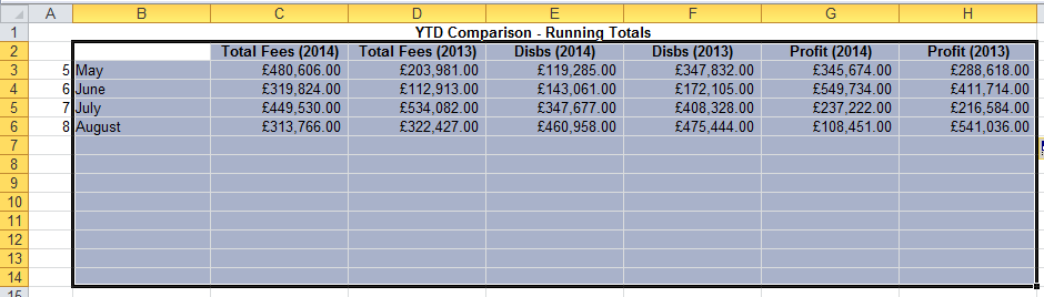
(Numbers randomized for public viewing). When September's figures are published, another row will be made 'visible', and so on until we reach April next year:
1bzAchP.png
 

Excel Facts

What is the shortcut key for Format Selection?
Ctrl+1 (the number one) will open the Format dialog for whatever is selected.
Try this:

1) In your formulas that return "", change them so that they return " " (a single space) instead.

2) In a hideable location (another tab, off to the right, whatever) put this formula:

=COUNTA(B:B)-COUNTIF(B:B," ")-1

This formula counts all of the non-blank values in that column, then subtracts a count of all of those that return " ", a single blank space. The additional -1 at the end adjusts for the header, but if you have other stuff in the same column, you may have to adjust.

3) Now you have a cell that counts the actual number of months you're showing. Use this in your OFFSET function as normal, and it should work fine.
 
Upvote 0
Thanks. Can you just confirm where in the OFFSET I use this new cell (with the COUNTA formula)?

Code:
=OFFSET(_Data![start]<start>:[end]<end>,1,0,COUNTA(_Data![start]<start>:[end]<end>)-1,1)
</end></start></end></start>
 
Upvote 0
You would use it in place of the COUNTA formula.

Code:
=OFFSET(_Data![start]:[end],1,0,[new cell reference],1)
 
Upvote 0
Yeah that's what I thought:

Code:
=OFFSET(_Data!$B$2:$H$14,1,0,_Data!$J$2,1)

J2 is where your formula is. This only selects column B though. Is it possible to get the dynamic range to select all the columns in my screenshot, without doing a separate dynamic range for each column? I have some other data with loadsa columns!

EDIT: Remembered that the last parameter for OFFSET is number of columns. Changing to 7 does what I need.

Thanks very much for your help. I shall definitely be using this in future projects :)
 
Last edited:
Upvote 0
PS: Is there any way to use a named range in a Chart without specifying the file name:

Code:
='File name.xlsx'!Range_Name

I have a 'working' file that gets saved as a different name for publishing... Does the file name reference change automatically when I do this, or just rename the file for example.
 
Upvote 0
Actually, the chart is not updating itself when another row is added, or made 'visible'. The Dynamic Range is working fine.

For the Chart:
Dyp15oQ.png


But when pressing OK, and going back to Select Data, it's changed itself to the 'fixed' range:
k6dd23r.png
 
Upvote 0
When using a dynamic range for a chart, make sure that the named range is defined at the worksheet level, not the workbook level. You should not have to include the workbook name when using the named range in a chart, but you will need to use the sheet name. Give that a shot, and I think it may address both of your recent posts.
 
Upvote 0
Thanks.

It doesn't seem to 'solve' the 2nd of my recent posts. You seem to have to edit each series in the chart to use a dynamic named range, rather than being able to set the whole chart to use a single dynamic named range.

Most online examples and videos all use the dynamic named ranges at the series level.

That's really, really poor design in my opinion. Terrible in fact. What if you had 50 columns, you'd have to have 50 dynamic named ranges, then manually update the 50 series' on the chart.

Once again, thanks for all your help.
 
Upvote 0
I see what you mean. Yes, it goes get pretty granular.

I don't know how useful this trick will be for you, but it may make the process of editing quicker. Create the chart based on a single static range, then select one of the data series in your chart (like for a bar chart, just click on one of the bars.) In the formula bar, you'll see a "SERIES" formula. The last argument in this formula should correspond to the location of your data. You can manually edit there to put in the dynamic range. You still have to do it one at a time, but there is less clicking through windows to get there.

Best of luck!
 
Upvote 0

Forum statistics

Threads
1,214,641
Messages
6,120,685
Members
448,977
Latest member
dbonilla0331

We've detected that you are using an adblocker.

We have a great community of people providing Excel help here, but the hosting costs are enormous. You can help keep this site running by allowing ads on MrExcel.com.
Allow Ads at MrExcel

Which adblocker are you using?

Disable AdBlock

Follow these easy steps to disable AdBlock

1)Click on the icon in the browser’s toolbar.
2)Click on the icon in the browser’s toolbar.
2)Click on the "Pause on this site" option.
Go back

Disable AdBlock Plus

Follow these easy steps to disable AdBlock Plus

1)Click on the icon in the browser’s toolbar.
2)Click on the toggle to disable it for "mrexcel.com".
Go back

Disable uBlock Origin

Follow these easy steps to disable uBlock Origin

1)Click on the icon in the browser’s toolbar.
2)Click on the "Power" button.
3)Click on the "Refresh" button.
Go back

Disable uBlock

Follow these easy steps to disable uBlock

1)Click on the icon in the browser’s toolbar.
2)Click on the "Power" button.
3)Click on the "Refresh" button.
Go back
Back
Top