Dynamic update of cell value based on color

[JLouis]

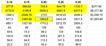
Hello. I have this range as shown below. This is a variety of price change options.

I need the user to be able to select a cell in F3:J3, the cell turn a color and the highlighted cell value to be displayed in K3. Repeat this down to row 16, and then add the selected cells together. I've tried some functions but they don't work dynamically and won't change when a new cell is selected. I hope I've explained this correctly. Thank you for your time.

1829.xlsm
	F	G	H	I	J	K
2	0.10	0.15	0.20	0.25	0.30
3	377.90	566.85	755.80	944.75	1133.70	377.9
4	2772.60	4158.90	5545.20	6931.50	8317.80
5	1366.50	2049.75	2733.00	3416.25	4099.50
6
7	977.30	1465.95	1954.60	2443.25	2931.90
8
9	885.10	1327.65	1770.20	2212.75	2655.30
10
11
12	64.00	96.00	128.00	160.00	192.00
13	49.60	74.40	99.20	124.00	148.80
14	104.60	156.90	209.20	261.50	313.80
15	56.60	84.90	113.20	141.50	169.80
16	22.20	33.30	44.40	55.50	66.60
17	6379.40	9569.10	12758.80	15948.50	19138.20
Price Increase Calcualtor

Cell Formulas
Range	Formula
F12:F16,F9,F7,F3:F5	F3	=E3*$F$2
G12:G16,G9,G7,G3:G5	G3	=E3*$G$2
H12:H16,H9,H7,H3:H5	H3	=E3*$H$2
I12:I16,I9,I7,I3:I5	I3	=E3*$I$2
J12:J16,J9,J7,J3:J5	J3	=E3*$J$2
K3	K3	=SumColor(K2,F3:J3)
F17:J17	F17	=SUM(F3:F9)

 

[maabadi]

For Selecting one Cell at each row try this Worksheet event code (Right Cilck on sheet name and then Select view code Then Paste code 1 or 2):
If you want Clear colors from Cells Select Cell K2.

Private Sub Worksheet_SelectionChange(ByVal Target As Range)
Dim i As Long, Lr As Long
Lr = Range("F" & Rows.Count).End(xlUp).Row
If Intersect(Target, Union(Range("F3:J" & Lr - 1), Range("K2"))) Is Nothing Then Exit Sub
If Target.Count > 1 Then Exit Sub
Application.EnableEvents = False
If Not Intersect(Target, Range("K2")) Is Nothing Then
Range("F3:J" & Lr - 1).Interior.Color = 16777215
Range("K2").Copy
Range("F3:J" & Lr - 1).PasteSpecial Paste:=xlPasteFormats, Operation:=xlNone, SkipBlanks:=False, Transpose:=False
Range("K3:K" & Lr - 1).ClearContents
Range("K2").Activate
End If
If Not Intersect(Target, Range("F3:J" & Lr - 1)) Is Nothing Then
Target.Interior.Color = 65535
Range("K" & Target.Row).Value = Target.Value
End If
Application.EnableEvents = True
End Sub

For Select Multiple Cell from Each row:

Private Sub Worksheet_SelectionChange(ByVal Target As Range)
Dim i As Long, Lr As Long, j As Long, K As Double
Lr = Range("F" & Rows.Count).End(xlUp).Row
If Intersect(Target, Union(Range("F3:J" & Lr - 1), Range("K2"))) Is Nothing Then Exit Sub
If Target.Count > 1 Then Exit Sub
Application.EnableEvents = False
If Not Intersect(Target, Range("K2")) Is Nothing Then
Range("F3:J" & Lr - 1).Interior.Color = 16777215
Range("K2").Copy
Range("F3:J" & Lr - 1).PasteSpecial Paste:=xlPasteFormats, Operation:=xlNone, SkipBlanks:=False, Transpose:=False
Range("K3:K" & Lr - 1).ClearContents
Range("K2").Activate
End If
If Not Intersect(Target, Range("F3:J" & Lr - 1)) Is Nothing Then
Target.Interior.Color = 65535
For j = 6 To 10
If Cells(Target.Row, j).Interior.Color = 65535 Then K = K + Cells(Target.Row, j).Value
Next j
Range("K" & Target.Row).Value = K
End If
Application.EnableEvents = True
End Sub

 

[JLouis]

Thank you so much for the reply. As far as I can tell, both codes do the exact same thing as far as the behavior of the sheet. The range f3:j12 work correctly and the selected cell updates correctly and dynamically.

There are two issues with the code. One is you can select more than one cell within the row. This was true with both formulas. The 2nd issue is that you can select and color cells outside of the range f3:j12.

Any suggestions on tweaking the code to address those two issues?

Thanks again for the assistance.

 

[JLouis]

Thank you so much for the reply. As far as I can tell, both codes do the exact same thing as far as the behavior of the sheet. The range f3:j12 work correctly and the selected cell updates correctly and dynamically.

There are two issues with the code. One is you can select more than one cell within the row. This was true with both formulas. The 2nd issue is that you can select and color cells outside of the range f3:j12.

Any suggestions on tweaking the code to address those two issues?

Thanks again for the assistance.

EDIT: I have solved the 2nd issue by relocating some cells being used under the shown range, making the lr-1 work correctly.

 

[JLouis]

EDIT: I have solved the 2nd issue by relocating some cells being used under the shown range, making the lr-1 work correctly.

EDIT: So the WB now works correctly. I added my previous effort to your work and although not great technique, the end result works just fine. I marked the question solved. Here's the code, don't laugh...



Private Sub Worksheet_SelectionChange(ByVal Target As Range)
Dim i As Long, Lr As Long
Static Cl As Range
Static C2 As Range
Static C3 As Range
Static C4 As Range
Static C5 As Range
Static C6 As Range
Static C7 As Range
Static C8 As Range
Static C9 As Range
Static C10 As Range
If Not Intersect(Target, Range("f3:j3")) Is Nothing Then
If Not Cl Is Nothing Then Cl.Interior.ColorIndex = 0
Set Cl = Target
End If
'2
If Not Intersect(Target, Range("f4:j4")) Is Nothing Then
If Not C2 Is Nothing Then C2.Interior.ColorIndex = 0
Set C2 = Target
End If
'3
If Not Intersect(Target, Range("f5:j5")) Is Nothing Then
If Not C3 Is Nothing Then C3.Interior.ColorIndex = 0
Set C3 = Target
End If
'4
If Not Intersect(Target, Range("f6:j6")) Is Nothing Then
If Not C4 Is Nothing Then C4.Interior.ColorIndex = 0
Set C4 = Target
End If
'5
If Not Intersect(Target, Range("f7:j7")) Is Nothing Then
If Not C5 Is Nothing Then C5.Interior.ColorIndex = 0
Set C5 = Target
End If
'6
If Not Intersect(Target, Range("f8:j8")) Is Nothing Then
If Not C6 Is Nothing Then C6.Interior.ColorIndex = 0
Set C6 = Target
End If
'7
If Not Intersect(Target, Range("f9:j9")) Is Nothing Then
If Not C7 Is Nothing Then C7.Interior.ColorIndex = 0
Set C7 = Target
End If
'8
If Not Intersect(Target, Range("f10:j10")) Is Nothing Then
If Not C8 Is Nothing Then C8.Interior.ColorIndex = 0
Set C8 = Target
End If
'9
If Not Intersect(Target, Range("f11:j11")) Is Nothing Then
If Not C9 Is Nothing Then C9.Interior.ColorIndex = 0
Set C9 = Target
End If
'10
If Not Intersect(Target, Range("f12:j12")) Is Nothing Then
If Not C10 Is Nothing Then C10.Interior.ColorIndex = 0
Set C10 = Target
End If
Lr = Range("F" & Rows.Count).End(xlUp).Row
If Intersect(Target, Union(Range("F3:J" & Lr - 1), Range("K2"))) Is Nothing Then Exit Sub
If Target.Count > 1 Then Exit Sub
Application.EnableEvents = False
If Not Intersect(Target, Range("K2")) Is Nothing Then
Range("F3:J" & Lr - 1).Interior.Color = 16777215
Range("K2").Copy
Range("F3:J" & Lr - 1).PasteSpecial Paste:=xlPasteFormats, Operation:=xlNone, SkipBlanks:=False, Transpose:=False
Range("K3:K" & Lr - 1).ClearContents
Range("K2").Activate
End If
If Not Intersect(Target, Range("F3:J" & Lr - 1)) Is Nothing Then
Target.Interior.Color = 65535
Range("K" & Target.Row).Value = Target.Value
End If
Application.EnableEvents = True
End Sub

 

[maabadi]

if you want add column C to Color & Sum it Values to K column, this is code:

Private Sub Worksheet_SelectionChange(ByVal Target As Range)
Dim i As Long, Lr As Long, j As Long, K As Double
Lr = Range("F" & Rows.Count).End(xlUp).Row
If Intersect(Target, Union(Range("C3:C" & Lr - 1), Range("F3:J" & Lr - 1), Range("K2"))) Is Nothing Then Exit Sub
If Target.Count > 1 Then Exit Sub
Application.EnableEvents = False
If Not Intersect(Target, Range("K2")) Is Nothing Then
Range("F3:J" & Lr - 1).Interior.Color = 16777215
Range("K2").Copy
Range("F3:J" & Lr - 1).PasteSpecial Paste:=xlPasteFormats, Operation:=xlNone, SkipBlanks:=False, Transpose:=False
Range("K3:K" & Lr - 1).ClearContents
Range("K2").Activate
End If
If Not Intersect(Target, Union(Range("C3:C" & Lr - 1), Range("F3:J" & Lr - 1))) Is Nothing Then
Target.Interior.Color = 65535
For j = 3 To 10
If Cells(Target.Row, j).Interior.Color = 65535 Then K = K + Cells(Target.Row, j).Value
if j = 3 Then j = j + 2
Next j
Range("K" & Target.Row).Value = K
End If
Application.EnableEvents = True
End Sub

 

[maabadi]

if you want select multiple cell at one row also try this:

Private Sub Worksheet_SelectionChange(ByVal Target As Range)
Dim i As Long, Lr As Long, j As Long, K As Double
Lr = Range("F" & Rows.Count).End(xlUp).Row
If Intersect(Target, Union(Range("C3:C" & Lr - 1), Range("F3:J" & Lr - 1), Range("K2"))) Is Nothing Then Exit Sub
Application.EnableEvents = False
Debug.Print Application.WorksheetFunction.Sum(Target)
If Not Intersect(Target, Range("K2")) Is Nothing Then
Range("F3:J" & Lr - 1).Interior.Color = 16777215
Range("K2").Copy
Range("F3:J" & Lr - 1).PasteSpecial Paste:=xlPasteFormats, Operation:=xlNone, SkipBlanks:=False, Transpose:=False
Range("K3:K" & Lr - 1).ClearContents
Range("K2").Activate
End If
If Not Intersect(Target, Union(Range("C3:C" & Lr - 1), Range("F3:J" & Lr - 1))) Is Nothing Then
Target.Interior.Color = 65535
For j = 3 To 10
If Cells(Target.Row, j).Interior.Color = 65535 Then K = K + Cells(Target.Row, j).Value
If j = 3 Then j = j + 2
Next j
Range("K" & Target.Row).Value = K
End If
Application.EnableEvents = True
End Sub

 

[JLouis]

Thank for all your help. The code is working perfectly.

 

[maabadi]

You're Welcome & Thanks for Feedback.