Dynamic VBA ranking

[anton05]

Hey Guys

I am new at MrExcel and hope you could help me out

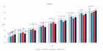
I have a spreadsheet where I in VBA determines a range, design, etc. to update and change a graph given the input selected in the tab. As it can be seen in this example from the screenshot the columns are simply listed based on the sequence the headings (brands) are listed in from the range.

I am looking to find a solution (a VBA code) to add where I dynamically can rank the brands descending after size in the given years (here just named data 1,2,3..)This means i would like it to look so that the number one is farthest to the left, then number two, number three and then at last number four to the right at each category (for the visualization/above screenshot, I have marked the columns in each category with 1-4 from largest to smallest).

I have tried to add the current VBA code(s) below:

Sub ParameterVælger()
    
    Application.ScreenUpdating = False
    
    Sheets("Data").Select

    Cells.Select
    Selection.EntireColumn.Hidden = False
    Selection.EntireRow.Hidden = False

    Dim MyCell As Range, MyRange As Range

Set MyRange = Range("B1:J1")
    
    For Each MyCell In MyRange
    If MyCell = False Then
    MyCell.EntireColumn.Hidden = True
        
    End If
    Next MyCell

Application.ScreenUpdating = True

End Sub

Sub Søjlegrafer_Vælger()

Application.ScreenUpdating = False

'Activates the other VBA's, which will hide the columns in the charts
     
 Call ParameterVælger
 
  For Each ch In Sheets("Choice").ChartObjects
    ch.Delete

Next ch

Worksheets("Graph").ChartObjects("Chart 2").Activate
ActiveChart.SetSourceData Source:=Range("'Data'!$B$3:$J$12")


'Changing chart to line diagram
ActiveChart.ChartType = 51

'Setting the size of the chart
Worksheets("Graph").Shapes("Chart 2").ScaleHeight 1, msoFalse, msoScaleFromTopLeft
Worksheets("Graph").Shapes("Chart 2").ScaleWidth 1, msoFalse, msoScaleFromTopLeft

'Remove outer gridline and make invisible
Worksheets("Graph").Shapes("Chart 2").Line.Visible = msoFalse
Worksheets("Graph").Shapes("Chart 2").Fill.Visible = msoFalse

'Add data labels and color for columns
ActiveChart.SetElement (msoElementDataLabelOutSideEnd)
ActiveChart.ChartGroups(1).GapWidth = 120
ActiveChart.ChartGroups(1).Overlap = -20
'Add Legend
ActiveChart.SetElement (msoElementLegendBottom)

'Add X-axis and adjust layout
Worksheets("Graph").ChartObjects("Chart 2").Chart.HasAxis(xlCategory, xlPrimary) = True
Worksheets("Graph").ChartObjects("Chart 2").Chart.Axes(xlCategory).ReversePlotOrder = False
  
'Add X-axis title and adjust layout
Worksheets("Graph").ChartObjects("Chart 2").Chart.Axes(xlCategory, xlPrimary).HasTitle = True
Worksheets("Graph").ChartObjects("Chart 2").Chart.Axes(xlCategory, xlPrimary).AxisTitle.Characters.Text = "Data"
  
'Add y-axis and adjust layout
Worksheets("Graph").ChartObjects("Chart 2").Chart.HasAxis(xlValue, xlPrimary) = True
Worksheets("Graph").ChartObjects("Chart 2").Chart.Axes(xlValue).MinimumScale = 80
Worksheets("Graph").ChartObjects("Chart 2").Chart.Axes(xlValue).MaximumScaleIsAuto = True
Worksheets("Graph").ChartObjects("Chart 2").Chart.Axes(xlValue).MajorUnit = 20
Worksheets("Graph").ChartObjects("Chart 2").Chart.Axes(xlValue).TickLabelPosition = xlNextToAxis
Worksheets("Graph").ChartObjects("Chart 2").Chart.Axes(xlValue).TickLabels.NumberFormat = "0"
  
'Add y-axis title and adjust layout
Worksheets("Graph").ChartObjects("Chart 2").Chart.Axes(xlValue, xlPrimary).HasTitle = True
Worksheets("Graph").ChartObjects("Chart 2").Chart.Axes(xlValue, xlPrimary).AxisTitle.Characters.Text = "Index"
  
'Add Major Gridlines horizontal and removes the vertical
Worksheets("Graph").ChartObjects("Chart 2").Chart.SetElement (msoElementPrimaryValueGridLinesMajor)
Worksheets("Graph").ChartObjects("Chart 2").Chart.SetElement (msoElementPrimaryCategoryGridLinesNone)

'Ensure chart has a title
Worksheets("Graph").ChartObjects("Chart 2").Chart.HasTitle = True

'Change chart's title
Worksheets("Graph").ChartObjects("Chart 2").Chart.ChartTitle.Text = "Graph 1"

Application.ScreenUpdating = True

'Copies chart and paste it in the "Choice" tab
Worksheets("Graph").ChartObjects("Chart 2").Activate
ActiveChart.ChartArea.Copy
Worksheets("Choice").Select
Range("E5").Select
ActiveSheet.Paste
Range("A1").Select

End Sub

I will be happy to share the workbook as well - please let me know if it is needed

I look forward to hearing your solutions.

Thank you so much in advance.

Anton