Dynamically Add rows based on formula

[tpexcelst]

Hello,
I am trying to figure out how to add a column, with a variable number of rows, based on the outcome of a formula.

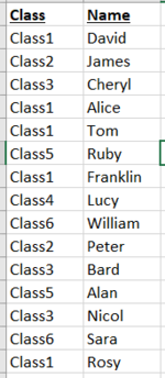
Im able to get from this data:

To this:

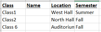
But the step I need help with is getting the information from the second table into the final table which looks like this:

I would need to add a certain number of rows depending on how many names are added to Column B. So for Class1 I would need to add 5 rows, Class2 2 rows, Class6 2 rows, etc.

What formula would I use in B2, B3, B4 to pull in the correct names and automatically add each name to a new row so that the final table looks like this?

Thank you!

 

[alansidman]

We cannot work with pictures, so using XL2BB, please upload your sample data and sample solution so that we can manipulate the data without having to recreate your worksheet. This appears to be a Power Query join of tables solution but will need your data to test.

 

[maabadi]

Welcome to MrExcel Message Board.
If your first image data is in Sheet2 Columns A:B
AND you want your Result Table Sheet3 Columns A:D
Try this:

Sub AddRowsBasedClass()
Dim i As Long
Dim j As Long
Dim n As Long
Dim Lr As Long
Dim Myrange As Range
Dim Myrange2 As Range
Dim Cell As Range
Lr = Sheets("Sheet2").Cells(Rows.Count, 2).End(xlUp).Row
Set Myrange = Sheets("Sheet2").Range("A1:B" & Lr)
Set Myrange2 = Sheets("Sheet3").Range("A1:D" & Lr)
Myrange.Sort key1:=Sheets("Sheet2").Columns("A"), Order1:=xlAscending, Key2:=Sheets("Sheet2").Columns("B"), Order2:=xlAscending, Header:=xlYes
Myrange2.Sort key1:=Sheets("Sheet3").Columns("A"), Order1:=xlAscending, Key2:=Sheets("Sheet3").Columns("B"), Order2:=xlAscending, Header:=xlYes


For i = 2 To Lr
For Each Cell In Sheets("Sheet2").Range("A2:A" & Lr)
If Sheets("Sheet3").Range("A" & i).Value = Cell.Value And Sheets("Sheet3").Range("A" & i).Value <> "" And Cell.Value <> Cell.Offset(-1, 0).Value Then
n = Application.WorksheetFunction.CountIf(Myrange, Cell)
If n <> 1 Then
Sheets("sheet3").Rows(i + 1).Resize(n - 1).Insert
End If
End If
Sheets("Sheet3").Range("B" & i).Value = Sheets("Sheet2").Range("B" & i).Value
Next Cell
Next i
End Sub

 

[tpexcelst]

We cannot work with pictures, so using XL2BB, please upload your sample data and sample solution so that we can manipulate the data without having to recreate your worksheet. This appears to be a Power Query join of tables solution but will need your data to test.

Hi @alansidman,
I downloaded xl2bb and have put my data here

Table 1

mrexcelquestion.xlsx
	D	E
1	Class	Name
2	Class1	David
3		Alice
4		Tom
5		Franklin
6		Rosy
7	Class2	James
8		Peter
9	Class 6	William
10		Sara
11	Class3	Cheryl
12		Bard
13		Nicol
Sheet1

Table 2

mrexcelquestion.xlsx
	A	B	C	D
1	Class	Name	Location	Semester
2	Class1		West Hall	Summer
3	Class2		North Hall	Fall
4	Class6		Auditorium	Fall
Sheet2

Table 3

mrexcelquestion.xlsx
	A	B	C	D
1	Class	Name	Location	Semester
2	Class1	David	West Hall	Summer
3		Alice
4		Tom
5		Franklin
6		Rosy
7	Class2	James	North Hall	Fall
8		Peter
9	Class6	William	Auditorium	Fall
10		Sara
Sheet3

Id like to take the information in table 1, and combine it with table 2, so that table 2 looks like table 3 as the final output.

 

[tpexcelst]

Welcome to MrExcel Message Board.
If your first image data is in Sheet2 Columns A:B
AND you want your Result Table Sheet3 Columns A:D
Try this:

Sub AddRowsBasedClass()
Dim i As Long
Dim j As Long
Dim n As Long
Dim Lr As Long
Dim Myrange As Range
Dim Myrange2 As Range
Dim Cell As Range
Lr = Sheets("Sheet2").Cells(Rows.Count, 2).End(xlUp).Row
Set Myrange = Sheets("Sheet2").Range("A1:B" & Lr)
Set Myrange2 = Sheets("Sheet3").Range("A1:D" & Lr)
Myrange.Sort key1:=Sheets("Sheet2").Columns("A"), Order1:=xlAscending, Key2:=Sheets("Sheet2").Columns("B"), Order2:=xlAscending, Header:=xlYes
Myrange2.Sort key1:=Sheets("Sheet3").Columns("A"), Order1:=xlAscending, Key2:=Sheets("Sheet3").Columns("B"), Order2:=xlAscending, Header:=xlYes


For i = 2 To Lr
For Each Cell In Sheets("Sheet2").Range("A2:A" & Lr)
If Sheets("Sheet3").Range("A" & i).Value = Cell.Value And Sheets("Sheet3").Range("A" & i).Value <> "" And Cell.Value <> Cell.Offset(-1, 0).Value Then
n = Application.WorksheetFunction.CountIf(Myrange, Cell)
If n <> 1 Then
Sheets("sheet3").Rows(i + 1).Resize(n - 1).Insert
End If
End If
Sheets("Sheet3").Range("B" & i).Value = Sheets("Sheet2").Range("B" & i).Value
Next Cell
Next i
End Sub

hi, would I just put this code into each cell ?

 

[maabadi]

Are you don't familiar with VBA? Hold ALT key and Press F11 . Then go to Insert menu, Module and Paste Code at right window.
Then Hit Play Key (Green small right arrow) at the Above of window and run it. (or back to Excel Window, Save as file as .xlsm (Macro-enabled Workbook). Then Go to View Tab, Select Last item, Macros, then View Macros, Select AddRowsBasedClass and Run.
Now your table is ready.

 

[alansidman]

With Power Query, bring each table into the Power Query Editor. PQ is called Get and Transform in 365 and is located on the Data Tab.

Once you have each table in Power Query, then join the two tables with a Left Outer Join. Here is the Mcode for that

let
    Source = Table.NestedJoin(Table1, {"Class"}, Table3, {"Class"}, "Table3", JoinKind.LeftOuter),
    #"Expanded Table3" = Table.ExpandTableColumn(Source, "Table3", {"Location", "Semester"}, {"Location", "Semester"})
in
    #"Expanded Table3"

and your end result looks like the following

Book2
	A	B	C	D
1	Class	Name	Location	Semester
2	Class1	David	West Hall	Summer
3	Class1	Alice	West Hall	Summer
4	Class1	Tom	West Hall	Summer
5	Class1	Franklin	West Hall	Summer
6	Class1	Rosy	West Hall	Summer
7	Class2	James	North Hall	Fall
8	Class2	Peter	North Hall	Fall
9	Class6	William	Auditorium	Fall
10	Class6	Sara	Auditorium	Fall
11	Class3	Cheryl
12	Class3	Bard
13	Class3	Nicol
Merge1

Your Mcode for table 1 before merging is

let
    Source = Excel.CurrentWorkbook(){[Name="Table1"]}[Content],
    #"Filled Down" = Table.FillDown(Source,{"Class"})
in
    #"Filled Down"