Dynamically find the end of range - by Resize

[RAJESH1960]

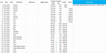
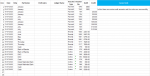
This data is sorted by Voucher Type and Credit. I want to count the number of rows with value in column Credit and select the same number of rows in column Particulars in the same sheet and copy. I am able to do that perfectly with the code written in the sheet but if the count of number of rows changes in a different sheet, it selects the same number of rows. I have no knowledge of how to resize the same number of rows in the 2 different columns. This is the code that works in this sheet only
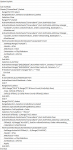
Option Explicit

Sub test()
'
' test Macro
'

'
Range("E2:F2").Select
Range(Selection, Selection.End(xlDown)).Select
Selection.Clear
Range("B2").Select
ActiveWorkbook.Worksheets("Canara Bank").Sort.SortFields.Clear
ActiveWorkbook.Worksheets("Canara Bank").Sort.SortFields.Add2 Key:=Range( _
"G2:G48"), SortOn:=xlSortOnValues, Order:=xlAscending, DataOption:= _
xlSortNormal
ActiveWorkbook.Worksheets("Canara Bank").Sort.SortFields.Add2 Key:=Range( _
"J2:J48"), SortOn:=xlSortOnValues, Order:=xlAscending, DataOption:= _
xlSortNormal
With ActiveWorkbook.Worksheets("Canara Bank").Sort
.SetRange Range("A1:K48")
.Header = xlYes
.MatchCase = False
.Orientation = xlTopToBottom
.SortMethod = xlPinYin
.Apply
End With
Range("J2").Select
Range(Selection, Selection.End(xlDown)).Select
Range("D2:J21").Select
Range("J2").Activate
Selection.Copy
Range("M2").Select
ActiveSheet.Paste
Range("M2").Select
Range(Selection, Selection.End(xlDown)).Select
Application.CutCopyMode = False
Selection.Copy
Range("E2").Select
ActiveSheet.Paste
Selection.End(xlDown).Select
ActiveCell.Offset(1, -1).Range("A1").Select
Range(Selection, Selection.End(xlDown)).Select
Application.CutCopyMode = False
Selection.Copy
Range("F22").Select
ActiveSheet.Paste
Application.CutCopyMode = False
Range("D2:F2").Select
Range(Selection, Selection.End(xlDown)).Select
Selection.SpecialCells(xlCellTypeBlanks).Select
Application.CutCopyMode = False
Selection.FormulaR1C1 = "=R1C11"
Range("M2:M3").Select
Range(Selection, Selection.End(xlDown)).Select
Range("M2:T21").Select
Selection.Clear
Range("A2").Select
ActiveWorkbook.Worksheets("Canara Bank").Sort.SortFields.Clear
ActiveWorkbook.Worksheets("Canara Bank").Sort.SortFields.Add2 Key:=Range( _
"A2:A48"), SortOn:=xlSortOnValues, Order:=xlAscending, DataOption:= _
xlSortNormal
With ActiveWorkbook.Worksheets("Canara Bank").Sort
.SetRange Range("A1:K48")
.Header = xlYes
.MatchCase = False
.Orientation = xlTopToBottom
.SortMethod = xlPinYin
.Apply
End With
Columns("E:F").Select
Columns("E:F").EntireColumn.AutoFit
Range("B2").Select
End Sub

 

[MARK858]

Actually what you ask doesn't make sense.
If the entire range in D2:D is empty then copy the range D2:D.

But D2:D is empty

 

[RAJESH1960]

Actually what you ask doesn't make sense.
If the entire range in D2:D is empty then copy the range D2:D.

But D2:D is empty

Mark. We are almost there. Let’s stay together. Remember we have used the auto filter function to filter the entries

Selection.AutoFilter

ActiveSheet.Range("$A$1:$K$236").AutoFilter Field:=7, Criteria1:="Contra"

ActiveSheet.Range("$A$1:$K$236").AutoFilter Field:=10, Criteria1:="<>"

Range("D2").Select

With Range("D2:D" & Range("D" & Rows.Count).End(xlUp).Row)

.Copy .Cells(1).Offset(, 1)

.Cells(1).Offset(, 1).AutoFilter

.Cells(.Rows.Count).Offset(1).Select

End With

If there are no entries at all then I don’t have to select - With Range("D2:D" & Range("D" & Rows.Count).End(xlUp).Row)

Then the auto filter is removed herein the code - .Cells(1).Offset(, 1).AutoFilter

So before Selecting - Range("D2").Select, I have to put an If function saying that if the Cell D2 is blank then remove filter and then - With Range("D2:D" & Range("D" & Rows.Count).End(xlUp).Row)

 

[MARK858]

So the range isn't empty. A range covers visible and non-visible cells.
You need to be more careful with your wording when asking questions.

 

[RAJESH1960]

So the range isn't empty. A range covers visible and non-visible cells.
You need to be more careful with your wording when asking questions.

After auto filter If the range is empty then it shouldn't copy or paste anything. That is why I need an If function also to be written in the code wherever necessary. I am trying my best to explain.

 

[MARK858]

Let's be clear if there is nothing in the whole range visible or not? then you want nothing to happen.
If D2 is empty but there is data either visible or not you want it unhidden and the whole range copied.
If D2 isn't empty then you want the visble D2:D range copied.

And this is all to happen before the Range("D2").Select (I would normally say about using Select but I am not going to rewrite the code today).

 

[RAJESH1960]

Let's be clear if there is nothing in the whole range visible or not? then you want nothing to happen.
If D2 is empty but there is data either visible or not you want it unhidden and the whole range copied.
If D2 isn't empty then you want the visble D2:D range copied.

And this is all to happen before the Range("D2").Select (I would normally say about using Select but I am not going to rewrite the code today).

If D2 is not empty then it has to copy the visible range by using that formula -
With Range("D2:D" & Range("D" & Rows.Count).End(xlUp).Row)
.Copy .Cells(1).Offset(, 1)
.Cells(1).Offset(, 1).AutoFilter
.Cells(.Rows.Count).Offset(1).Select
End With
Range(Selection, Selection.End(xlDown)).Select
Selection.Copy
and the rest of the code follows...

If D2 is empty, I remove the auto filter option and that displays the whole data. Then only the range is visible. Then I have to use the formula -
With Range("D2:D" & Range("D" & Rows.Count).End(xlUp).Row)
.Copy .Cells(1).Offset(, 1)
.Cells(1).Offset(, 1).AutoFilter
.Cells(.Rows.Count).Offset(1).Select
End With
Range(Selection, Selection.End(xlDown)).Select
Selection.Copy
Manually it is possible and this is a regular procedure to be followed. So, I thought why not use a VBA macro to do it. Its is almost done. Only the part where there are no visible cells in D2 after applying the auto filter option, needs a code.

 

[RAJESH1960]

The code has to run in the sheet with different data which will have different number of entries. I am sending you 2 different sheets. If the code runs in both the sheets without mistake then that is it.

 

[RAJESH1960]

I checked online and edited the code. It runs successfully where there are no contra > Credit entries. The code doesn't run if there are contra > credit entries. Now You can combine both the codes which are running successfully in 2 different sheets. I tried combining both but was not able to do it.

 

[MARK858]

I am leaving this post as I ask some simple questions for clarity expecting some straightforward answers and instead rather than straightforward answers you give me more images and more amended code.

 

[RAJESH1960]

I am leaving this post as I ask some simple questions for clarity expecting some straightforward answers and instead rather than straightforward answers you give me more images and more amended code.

Sorry Mark, Even I have given up on this. Thanks for your time.