Excel Calculation using VBA

[oHoi99]

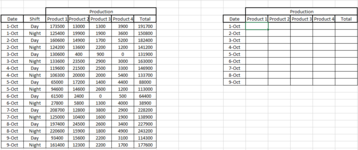
Hi.. does anyone know how to calculate the values automatically using VBA..? For example for Cell Z13, the calculation is Q13+Q14, and for Z14, the calculation is Q15+Q16, and so on...
I've been thinking how to do the calculation but still cant figure it out. Could anyone send some help here, please?

 

[pjmorris]

You don't need to create a formula, simply go click on a cell in your source table, then click on Insert Pivottable on the Insert Menu. Then choose dates as the Row component and put Products in the Values area.

It'll give you exactly what you need.

HTH

 

[oHoi99]

You don't need to create a formula, simply go click on a cell in your source table, then click on Insert Pivottable on the Insert Menu. Then choose dates as the Row component and put Products in the Values area.

It'll give you exactly what you need.

HTH

Oh, why didn't I think of that one. Thanks pjmorris!

 

[pjmorris]

its a pleasure

 

[mohadin]

Any Way

Sub test()
    Dim i, ii
    ii = 13
    For i = 13 To Cells(Rows.Count, "Q").End(xlUp).Row Step 2
        Range("Z" & ii) = Range("Q" & i) + Range("Q" & i + 1)
        ii = ii + 1
    Next
End Sub

 

[oHoi99]

Any Way

Sub test()
    Dim i, ii
    ii = 13
    For i = 13 To Cells(Rows.Count, "Q").End(xlUp).Row Step 2
        Range("Z" & ii) = Range("Q" & i) + Range("Q" & i + 1)
        ii = ii + 1
    Next
End Sub

Hi Mohadin,

Thank you very much! Very much appreciated

 

[Phuoc]

Try this in Z13:

=SUMIF($O$13:$O$30,$I13,INDEX($Q$13:$T$30,0,MATCH(Z$12,$Q$12:$T$12,0)))

 

[oHoi99]

Try this in Z13:

=SUMIF($O$13:$O$30,$I13,INDEX($Q$13:$T$30,0,MATCH(Z$12,$Q$12:$T$12,0)))

Thanks! Will try it out

 

[Dossfm0q]

what about

Yyy.xlsx
	A	B	C	D	E	F	G	H	I	J	K	L	M	N
1			Production							Production
2	Date	Shift	Product 1	Product	Product3	Product4	Total		Date	Productl	Product2	Product3	Product4	Total
3	01-Oct	Day	173500	13000	1300	3900	191700		01-Oct	298900	32900	3200	7500	342500
4	02-Oct	Night	125400	19900	1900	3600	150800		02-Oct	284800	28500	3900	6400	323600
5	02-Oct	Day	160600	14900	1700	5200	182400		03-Oct	264200	23900	3800	3000	294900
6	02-Oct	Night	124200	13600	2200	1200	141200		04-Oct	225900	41500	4500	8700	280600
7	03-Oct	Day	130600	400	900	0	131900		05-Oct	159600	31800	4000	5600	201000
8	04-Oct	Night	133600	23500	2900	3000	163000		06-Oct	89300	8200	1300	4500	103300
9	04-Oct	Day	119600	21500	2500	3300	146900		07-Oct	333700	23200	5400	4800	367100
10	05-Oct	Night	106300	20000	2000	5400	133700		08-Oct	418000	40400	4400	8300	471100
11	05-Oct	Day	65000	17200	1400	4400	88000		09-Oct	254800	27900	4400	4800	291900
12	05-Oct	Night	94600	14600	2600	1200	113000
13	06-Oct	Day	61500	2400	0	500	64400
14	06-Oct	Night	27800	5800	1300	4000	38900
15	07-Oct	Day	208700	12800	3800	2900	228200
16	07-Oct	Night	125000	10400	1600	1900	138900
17	08-Oct	Day	197400	24500	2600	3400	227900
18	08-Oct	Night	220600	15900	1800	4900	243200
19	09-Oct	Day	93400	15600	2200	3100	114300
20	10-Oct	Night	161400	12300	2200	1700	177600
21
Sheet1

Cell Formulas
Range	Formula
J3:M11	J3	=SUM(OFFSET(INDIRECT(ADDRESS(((ROW()-ROW($J$3))*2)+ROW($C$3),COLUMN(C3))),0,0,2,1))
N3:N11	N3	=SUM(J3:M3)

Cells with Conditional Formatting
Cell	Condition		Cell Format	Stop If True
I3:N11	Expression	=MOD(ROW()-ROW($I$3)+1,2)<>0	text	NO
A3:G20	Expression	=MOD(ROW()-ROW($A$3)+1,2)<>0	text	NO

Yyy.xlsx
	A	B	C	D	E	F	G	H	I	J	K	L	M	N
1
2
3
4
5
6
7
8
9
10
11			Production							Production
12	Date	Shift	Product 1	Product	Product3	Product4	Total		Date	Productl	Product2	Product3	Product4	Total
13	01-Oct	Day	173500	13000	1300	3900	191700		01-Oct	298900	32900	3200	7500	342500
14	02-Oct	Night	125400	19900	1900	3600	150800		02-Oct	284800	28500	3900	6400	323600
15	02-Oct	Day	160600	14900	1700	5200	182400		03-Oct	264200	23900	3800	3000	294900
16	02-Oct	Night	124200	13600	2200	1200	141200		04-Oct	225900	41500	4500	8700	280600
17	03-Oct	Day	130600	400	900	0	131900		05-Oct	159600	31800	4000	5600	201000
18	04-Oct	Night	133600	23500	2900	3000	163000		06-Oct	89300	8200	1300	4500	103300
19	04-Oct	Day	119600	21500	2500	3300	146900		07-Oct	333700	23200	5400	4800	367100
20	05-Oct	Night	106300	20000	2000	5400	133700		08-Oct	418000	40400	4400	8300	471100
21	05-Oct	Day	65000	17200	1400	4400	88000		09-Oct	254800	27900	4400	4800	291900
22	05-Oct	Night	94600	14600	2600	1200	113000
23	06-Oct	Day	61500	2400	0	500	64400
24	06-Oct	Night	27800	5800	1300	4000	38900
25	07-Oct	Day	208700	12800	3800	2900	228200
26	07-Oct	Night	125000	10400	1600	1900	138900
27	08-Oct	Day	197400	24500	2600	3400	227900
28	08-Oct	Night	220600	15900	1800	4900	243200
29	09-Oct	Day	93400	15600	2200	3100	114300
30	10-Oct	Night	161400	12300	2200	1700	177600
31
Sheet1

Cell Formulas
Range	Formula
J13:M21	J13	=SUM(OFFSET(INDIRECT(ADDRESS(((ROW()-ROW($J$13))*2)+ROW($C$13),COLUMN(C13))),0,0,2,1))
N13:N21	N13	=SUM(J13:M13)

Cells with Conditional Formatting
Cell	Condition		Cell Format	Stop If True
I13:N21	Expression	=MOD(ROW()-ROW($I$13)+1,2)<>0	text	NO
A13:G30	Expression	=MOD(ROW()-ROW($A$13)+1,2)<>0	text	NO

 

[oHoi99]

what about

Yyy.xlsx
	A	B	C	D	E	F	G	H	I	J	K	L	M	N
1			Production							Production
2	Date	Shift	Product 1	Product	Product3	Product4	Total		Date	Productl	Product2	Product3	Product4	Total
3	01-Oct	Day	173500	13000	1300	3900	191700		01-Oct	298900	32900	3200	7500	342500
4	02-Oct	Night	125400	19900	1900	3600	150800		02-Oct	284800	28500	3900	6400	323600
5	02-Oct	Day	160600	14900	1700	5200	182400		03-Oct	264200	23900	3800	3000	294900
6	02-Oct	Night	124200	13600	2200	1200	141200		04-Oct	225900	41500	4500	8700	280600
7	03-Oct	Day	130600	400	900	0	131900		05-Oct	159600	31800	4000	5600	201000
8	04-Oct	Night	133600	23500	2900	3000	163000		06-Oct	89300	8200	1300	4500	103300
9	04-Oct	Day	119600	21500	2500	3300	146900		07-Oct	333700	23200	5400	4800	367100
10	05-Oct	Night	106300	20000	2000	5400	133700		08-Oct	418000	40400	4400	8300	471100
11	05-Oct	Day	65000	17200	1400	4400	88000		09-Oct	254800	27900	4400	4800	291900
12	05-Oct	Night	94600	14600	2600	1200	113000
13	06-Oct	Day	61500	2400	0	500	64400
14	06-Oct	Night	27800	5800	1300	4000	38900
15	07-Oct	Day	208700	12800	3800	2900	228200
16	07-Oct	Night	125000	10400	1600	1900	138900
17	08-Oct	Day	197400	24500	2600	3400	227900
18	08-Oct	Night	220600	15900	1800	4900	243200
19	09-Oct	Day	93400	15600	2200	3100	114300
20	10-Oct	Night	161400	12300	2200	1700	177600
21
Sheet1

Cell Formulas
Range	Formula
J3:M11	J3	=SUM(OFFSET(INDIRECT(ADDRESS(((ROW()-ROW($J$3))*2)+ROW($C$3),COLUMN(C3))),0,0,2,1))
N3:N11	N3	=SUM(J3:M3)

Cells with Conditional Formatting
Cell	Condition		Cell Format	Stop If True
I3:N11	Expression	=MOD(ROW()-ROW($I$3)+1,2)<>0	text	NO
A3:G20	Expression	=MOD(ROW()-ROW($A$3)+1,2)<>0	text	NO

Yyy.xlsx
	A	B	C	D	E	F	G	H	I	J	K	L	M	N
1
2
3
4
5
6
7
8
9
10
11			Production							Production
12	Date	Shift	Product 1	Product	Product3	Product4	Total		Date	Productl	Product2	Product3	Product4	Total
13	01-Oct	Day	173500	13000	1300	3900	191700		01-Oct	298900	32900	3200	7500	342500
14	02-Oct	Night	125400	19900	1900	3600	150800		02-Oct	284800	28500	3900	6400	323600
15	02-Oct	Day	160600	14900	1700	5200	182400		03-Oct	264200	23900	3800	3000	294900
16	02-Oct	Night	124200	13600	2200	1200	141200		04-Oct	225900	41500	4500	8700	280600
17	03-Oct	Day	130600	400	900	0	131900		05-Oct	159600	31800	4000	5600	201000
18	04-Oct	Night	133600	23500	2900	3000	163000		06-Oct	89300	8200	1300	4500	103300
19	04-Oct	Day	119600	21500	2500	3300	146900		07-Oct	333700	23200	5400	4800	367100
20	05-Oct	Night	106300	20000	2000	5400	133700		08-Oct	418000	40400	4400	8300	471100
21	05-Oct	Day	65000	17200	1400	4400	88000		09-Oct	254800	27900	4400	4800	291900
22	05-Oct	Night	94600	14600	2600	1200	113000
23	06-Oct	Day	61500	2400	0	500	64400
24	06-Oct	Night	27800	5800	1300	4000	38900
25	07-Oct	Day	208700	12800	3800	2900	228200
26	07-Oct	Night	125000	10400	1600	1900	138900
27	08-Oct	Day	197400	24500	2600	3400	227900
28	08-Oct	Night	220600	15900	1800	4900	243200
29	09-Oct	Day	93400	15600	2200	3100	114300
30	10-Oct	Night	161400	12300	2200	1700	177600
31
Sheet1

Cell Formulas
Range	Formula
J13:M21	J13	=SUM(OFFSET(INDIRECT(ADDRESS(((ROW()-ROW($J$13))*2)+ROW($C$13),COLUMN(C13))),0,0,2,1))
N13:N21	N13	=SUM(J13:M13)

Cells with Conditional Formatting
Cell	Condition		Cell Format	Stop If True
I13:N21	Expression	=MOD(ROW()-ROW($I$13)+1,2)<>0	text	NO
A13:G30	Expression	=MOD(ROW()-ROW($A$13)+1,2)<>0	text	NO

Thanks a lot!