I am having trouble with my Q1 formula.....
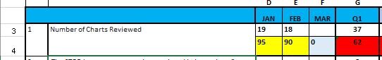
We tend to input the number of charts we have reviewed, in row 3 (Jan -17 charts, Feb -18 charts, etc)...
We are supposed to audit and review about 20 charts a month.
So for January, I see how we got 85% (we reviewed 17 charts out of 20, so 85%)
What I need help with is developing a quarterly formula, because right now, if I follow the same formula we set up below, for Q1 we get 58%, but that is not right, when we got 85% in Jan and 90% in Feb....
I thought about using an Average for Q1 (G4) but wasnt sure if that would be appropriate or accurate.
Is there a better formula to use to give you an accurate ongoing quarterly percentages?
When we input the number of charts for Jan, Feb & March, the quarterly numbers look accurate, it's when we are not done reviewing charts for 3 full months, that Q1 doesnt look accruate....
D E F G
| JAN | FEB | MAR | Q1 | |||
| 3 | Number of Charts Reviewed | 17 | 18 | SUM(D3:F3) = 35 | ||
| 4 | Percentage (based on maximum 20 charts) | D3/20*100 = 85 | E3/20*100 = 90 | F3/20*100 | G3/60*100 = 58 |