Excel Formula Question

Parebody

New Member
Joined
Jan 4, 2018
Messages
43
Office Version
  1. 2016
Platform
  1. Windows
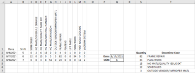
I'm looking for some assistance. I'm trying to create formula's in cell's S3 to T7 that will automatically pull data from the table on the left based on the date & shift entered into cell's Q3 & Q4. I would like the list generated to only show codes with data (no zero's), and I would like the list in ascending order by quantity (smallest to largest).
1630358520707.png
 

Attachments

  • 1630358058518.png
    1630358058518.png
    35.5 KB · Views: 4

Excel Facts

Which lookup functions find a value equal or greater than the lookup value?
MATCH uses -1 to find larger value (lookup table must be sorted ZA). XLOOKUP uses 1 to find values greater and does not need to be sorted.
You might run into issues with this mess of a formula.

ATG.xlsx
ABCDEFGHIJKLMNOPQRSTUVW
1DateShiftScheduledNo Matl/Sched ChangeNo Matl/ Quality IssueNo Matl/Material HandlerNo Matl/ExtrusionOutside Vendor/Improper MatlFrame RepairPlatensLift TablePlug WorkPost Mold CoolingVacuum System
28/16/202150261900401000
38/17/202161201500382003400QtyCodeAttributeValue
48/18/202170038560230001223Outside Vendor/Improper MatlOutside Vendor/Improper Matl3
5Date:8/17/202112ScheduledScheduled12
6Shift:615No Matl/ Quality IssueNo Matl/ Quality Issue15
734Plug WorkPlug Work34
882Frame RepairFrame Repair82
Sheet2
Cell Formulas
RangeFormula
A3:A4A3=A2+1
S4:S8S4=IFERROR(AGGREGATE(15,6,1/(INDEX($C$2:$N$4,SUMPRODUCT(($A$2:$A$4=$Q$5)*($B$2:$B$4=$Q$6)*ROW($A$2:$A$4))-ROW($A$1),0)<>0)*INDEX($C$2:$N$4,SUMPRODUCT(($A$2:$A$4=$Q$5)*($B$2:$B$4=$Q$6)*ROW($A$2:$A$4))-ROW($A$1),0),ROWS($A$1:A1)),"")
T4:T8T4=IFERROR(INDEX($C$1:$N$1,MATCH(S4,INDEX($C$2:$N$4,SUMPRODUCT(($A$2:$A$4=$Q$5)*($B$2:$B$4=$Q$6)*ROW($A$2:$A$4))-ROW($A$1),0),0)),"")


So, I would use Power Query instead.

Power Query:
let
    Source = Excel.CurrentWorkbook(){[Name="Table2"]}[Content],
    Type = Table.TransformColumnTypes(Source,{{"Date", type date}}),
    SR = Table.SelectRows(Type, each _[Date]=Date and _[Shift]=Shift),
    RC = Table.RemoveColumns(SR,{"Date", "Shift"}),
    Unpivot = Table.UnpivotOtherColumns(RC, {}, "Attribute", "Value"),
    Filter = Table.SelectRows(Unpivot, each ([Value] <> 0)),
    Sort = Table.Sort(Filter,{{"Value", Order.Ascending}})
in
    Sort

Code for Date and Shift

Power Query:
let
    Source = Excel.CurrentWorkbook(){[Name="Table1"]}[Content],
    Column2 = Date.From(Source{0}[Column2])
in
    Column2

Power Query:
let
    Source = Excel.CurrentWorkbook(){[Name="Table1"]}[Content],
    Column2 = Source{1}[Column2]
in
    Column2
 
Upvote 0
Another set of formulas that look to be a bit shorter:

Book4 (version 1).xlsb
ABCDEFGHIJKLMNOPQRST
1DateShiftScheduledNo MATL/SCHEDULE CHANGENO MATL/QUALITY ISSUE YETNO MATL/MATERIAL HANDLERNO MATL/EXTRUSIONOUTSIDE VENDOR/IMPROPER MATLFRAME REPAIRPLATENSLIFT TABLEPLUG WORKPOST MOLD COOLINGVACUUM SYSTEM
28/16/202150261900401000QuantityDowntime Code
38/17/202161201500382003400Date:8/17/20213OUTSIDE VENDOR/IMPROPER MATL
48/18/20217003856023000122Shift:612Scheduled
515NO MATL/QUALITY ISSUE YET
634PLUG WORK
782FRAME REPAIR
8  
9  
10  
Sheet1
Cell Formulas
RangeFormula
S3:S10S3=IFERROR(AGGREGATE(15,6,1/(1/($C$2:$N$4/($A$2:$A$4=$Q$3)/($B$2:$B$4=$Q$4))),ROWS($S$3:$S3)),"")
T3:T10T3=IF(S3="","",INDEX($1:$1,AGGREGATE(15,6,COLUMN($C$1:$N$1)/(INDEX($C$2:$N$4,MATCH($Q$3&"|"&$Q$4,$A$2:$A$4&"|"&$B$2:$B$4,0),0)=S3),COUNTIF($S$2:$S3,S3))))
 
Upvote 0
Solution
You might run into issues with this mess of a formula.

ATG.xlsx
ABCDEFGHIJKLMNOPQRSTUVW
1DateShiftScheduledNo Matl/Sched ChangeNo Matl/ Quality IssueNo Matl/Material HandlerNo Matl/ExtrusionOutside Vendor/Improper MatlFrame RepairPlatensLift TablePlug WorkPost Mold CoolingVacuum System
28/16/202150261900401000
38/17/202161201500382003400QtyCodeAttributeValue
48/18/202170038560230001223Outside Vendor/Improper MatlOutside Vendor/Improper Matl3
5Date:8/17/202112ScheduledScheduled12
6Shift:615No Matl/ Quality IssueNo Matl/ Quality Issue15
734Plug WorkPlug Work34
882Frame RepairFrame Repair82
Sheet2
Cell Formulas
RangeFormula
A3:A4A3=A2+1
S4:S8S4=IFERROR(AGGREGATE(15,6,1/(INDEX($C$2:$N$4,SUMPRODUCT(($A$2:$A$4=$Q$5)*($B$2:$B$4=$Q$6)*ROW($A$2:$A$4))-ROW($A$1),0)<>0)*INDEX($C$2:$N$4,SUMPRODUCT(($A$2:$A$4=$Q$5)*($B$2:$B$4=$Q$6)*ROW($A$2:$A$4))-ROW($A$1),0),ROWS($A$1:A1)),"")
T4:T8T4=IFERROR(INDEX($C$1:$N$1,MATCH(S4,INDEX($C$2:$N$4,SUMPRODUCT(($A$2:$A$4=$Q$5)*($B$2:$B$4=$Q$6)*ROW($A$2:$A$4))-ROW($A$1),0),0)),"")


So, I would use Power Query instead.

Power Query:
let
    Source = Excel.CurrentWorkbook(){[Name="Table2"]}[Content],
    Type = Table.TransformColumnTypes(Source,{{"Date", type date}}),
    SR = Table.SelectRows(Type, each _[Date]=Date and _[Shift]=Shift),
    RC = Table.RemoveColumns(SR,{"Date", "Shift"}),
    Unpivot = Table.UnpivotOtherColumns(RC, {}, "Attribute", "Value"),
    Filter = Table.SelectRows(Unpivot, each ([Value] <> 0)),
    Sort = Table.Sort(Filter,{{"Value", Order.Ascending}})
in
    Sort

Code for Date and Shift

Power Query:
let
    Source = Excel.CurrentWorkbook(){[Name="Table1"]}[Content],
    Column2 = Date.From(Source{0}[Column2])
in
    Column2

Power Query:
let
    Source = Excel.CurrentWorkbook(){[Name="Table1"]}[Content],
    Column2 = Source{1}[Column2]
in
    Column2
Thank you, this was very helpful!
 
Upvote 0
Another set of formulas that look to be a bit shorter:

Book4 (version 1).xlsb
ABCDEFGHIJKLMNOPQRST
1DateShiftScheduledNo MATL/SCHEDULE CHANGENO MATL/QUALITY ISSUE YETNO MATL/MATERIAL HANDLERNO MATL/EXTRUSIONOUTSIDE VENDOR/IMPROPER MATLFRAME REPAIRPLATENSLIFT TABLEPLUG WORKPOST MOLD COOLINGVACUUM SYSTEM
28/16/202150261900401000QuantityDowntime Code
38/17/202161201500382003400Date:8/17/20213OUTSIDE VENDOR/IMPROPER MATL
48/18/20217003856023000122Shift:612Scheduled
515NO MATL/QUALITY ISSUE YET
634PLUG WORK
782FRAME REPAIR
8  
9  
10  
Sheet1
Cell Formulas
RangeFormula
S3:S10S3=IFERROR(AGGREGATE(15,6,1/(1/($C$2:$N$4/($A$2:$A$4=$Q$3)/($B$2:$B$4=$Q$4))),ROWS($S$3:$S3)),"")
T3:T10T3=IF(S3="","",INDEX($1:$1,AGGREGATE(15,6,COLUMN($C$1:$N$1)/(INDEX($C$2:$N$4,MATCH($Q$3&"|"&$Q$4,$A$2:$A$4&"|"&$B$2:$B$4,0),0)=S3),COUNTIF($S$2:$S3,S3))))
Eric, what would I change to make the list Decsending (Largest to smallest)?
 
Upvote 0
Eric, what would I change to make the list Decsending (Largest to smallest)?

Just change the 15 to 14 in the S3 formula:

=IFERROR(AGGREGATE(14,6,1/(1/($C$2:$N$4/($A$2:$A$4=$Q$3)/($B$2:$B$4=$Q$4))),ROWS($S$3:$S3)),"")

The T3 formula doesn't change.
 
Upvote 0
Just change the 15 to 14 in the S3 formula:

=IFERROR(AGGREGATE(14,6,1/(1/($C$2:$N$4/($A$2:$A$4=$Q$3)/($B$2:$B$4=$Q$4))),ROWS($S$3:$S3)),"")

The T3 formula doesn't change.
Simple enough. Thanks Eric, you've been a huge help!
 
Upvote 0

Forum statistics

Threads
1,214,641
Messages
6,120,691
Members
448,978
Latest member
rrauni

We've detected that you are using an adblocker.

We have a great community of people providing Excel help here, but the hosting costs are enormous. You can help keep this site running by allowing ads on MrExcel.com.
Allow Ads at MrExcel

Which adblocker are you using?

Disable AdBlock

Follow these easy steps to disable AdBlock

1)Click on the icon in the browser’s toolbar.
2)Click on the icon in the browser’s toolbar.
2)Click on the "Pause on this site" option.
Go back

Disable AdBlock Plus

Follow these easy steps to disable AdBlock Plus

1)Click on the icon in the browser’s toolbar.
2)Click on the toggle to disable it for "mrexcel.com".
Go back

Disable uBlock Origin

Follow these easy steps to disable uBlock Origin

1)Click on the icon in the browser’s toolbar.
2)Click on the "Power" button.
3)Click on the "Refresh" button.
Go back

Disable uBlock

Follow these easy steps to disable uBlock

1)Click on the icon in the browser’s toolbar.
2)Click on the "Power" button.
3)Click on the "Refresh" button.
Go back
Back
Top