Excel formulas are not copying up

[dualwieldbacon]

Hi all.

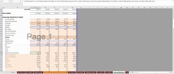
I'm trying to amalgamate two income statements into a separate worksheet for a 'combined income statement'. For some reason, when I try to copy my formulas into my target cells, the formula does not work.

The formula I am using in cell C59 is as follows:
=IFERROR(INDEX('IS-1482272'!$B$5:$G$96,MATCH($B59,'IS-1482272'!$B$5:$B$96,0),MATCH(C$5,'IS-1482272'!$B$5:$G$5,0))+INDEX('IS-2299824'!$B$5:$G$96,MATCH($B59,'IS-2299824'!$B$5:$B$96,0),MATCH(C$5,'IS-2299824'!$B$5:$G$5,0)),0)

This formula is used throughout my target worksheet, but it's not copying correctly into my rows 56 through 58 for some reason. My source data is located in sheets 'IS-1482272' and 'IS-2299824'. The sheet that the formulas are on is 'Income Statement'. I've gone into Formulas -> Calculation Options and I've made sure that 'Automatic' is selected.

Any thoughts??

 

[jasonb75]

Any thoughts??

None without seeing the formula in the cell that is not working, and without knowing how you're trying to copy the formula to the other cells.

It could be as simple as trailing spaces in B56:B58 on one of the sheets causing the whole thing to error.

The fact that the formulas in row 59 are working tells me that the column matches are working correctly, but that is the only definite factor that can be established so far.

 

[dualwieldbacon]

None without seeing the formula in the cell that is not working, and without knowing how you're trying to copy the formula to the other cells.

It could be as simple as trailing spaces in B56:B58 on one of the sheets causing the whole thing to error.

The fact that the formulas in row 59 are working tells me that the column matches are working correctly, but that is the only definite factor that can be established so far.

Here is the formula from C56: =IFERROR(INDEX('IS-1482272'!$B$5:$G$96,MATCH($B56,'IS-1482272'!$B$5:$B$96,0),MATCH(C$5,'IS-1482272'!$B$5:$G$5,0))+INDEX('IS-2299824'!$B$5:$G$96,MATCH($B56,'IS-2299824'!$B$5:$B$96,0),MATCH(C$5,'IS-2299824'!$B$5:$G$5,0)),0)

I copied the formula to the other cells by highlighting my selection from C59 to G59, then dragging the corner up in to the above 3 rows. I've tried deleting the cells in column B and retyping those accounts (Telephone, Travel, Utilities) but that didn't seem to fix it up.

 

[jasonb75]

That should work perfectly fine. If the values in the 2 source sheets are from formulas then I can see a potential problem in the event that one sheet had a value while the other was blank, but given that both sheets have values it should be giving you something.

If this gives you a result that is equal to the value from one of the sheets then that will identify a problem in the other sheet.

=IFERROR(INDEX('IS-1482272'!$B$5:$G$96,MATCH($B56,'IS-1482272'!$B$5:$B$96,0),MATCH(C$5,'IS-1482272'!$B$5:$G$5,0)),0)+IFERROR(INDEX('IS-2299824'!$B$5:$G$96,MATCH($B56,'IS-2299824'!$B$5:$B$96,0),MATCH(C$5,'IS-2299824'!$B$5:$G$5,0)),0)

To test for additional problems, try

=MATCH($B56,'IS-1482272'!$B$5:$B$96,0)+4

and

=MATCH($B56,'IS-2299824'!$B$5:$B$96,0)+4

Do they return errors or numbers? If they return numbers then that will tell you which row the result is coming from in the source sheets (possibly not the correct row). If they return errors then it means that for some reason that (Telephone, Travel, Utilities) in column B are still not matching correctly.

 

[dualwieldbacon]

That should work perfectly fine. If the values in the 2 source sheets are from formulas then I can see a potential problem in the event that one sheet had a value while the other was blank, but given that both sheets have values it should be giving you something.

If this gives you a result that is equal to the value from one of the sheets then that will identify a problem in the other sheet.

=IFERROR(INDEX('IS-1482272'!$B$5:$G$96,MATCH($B56,'IS-1482272'!$B$5:$B$96,0),MATCH(C$5,'IS-1482272'!$B$5:$G$5,0)),0)+IFERROR(INDEX('IS-2299824'!$B$5:$G$96,MATCH($B56,'IS-2299824'!$B$5:$B$96,0),MATCH(C$5,'IS-2299824'!$B$5:$G$5,0)),0)

To test for additional problems, try

=MATCH($B56,'IS-1482272'!$B$5:$B$96,0)+4

and

=MATCH($B56,'IS-2299824'!$B$5:$B$96,0)+4

Do they return errors or numbers? If they return numbers then that will tell you which row the result is coming from in the source sheets (possibly not the correct row). If they return errors then it means that for some reason that (Telephone, Travel, Utilities) in column B are still not matching correctly.

Fantastic! The second formula you gave me helped me identify the problem. It turns out that I have two rows within my source sheets with the heading 'Telephone' (and Travel and Utilities), which was confusing the original formula I had worked out.