Excel help for a novice

[sjohnson77]

Hi Guys,

In my current role I have to look at data for a financial year and change it into calendar year data.

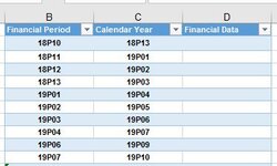
In my company, a financial year has 13 periods (4 weeks per period) and starts from April each year (e.g. 18P04 = 2018 Period 4).

The issue I am experiencing is that with P01 being from April, I need a way of converting the period data in calendar year data. So period 01 needs to become period 4 (+3 months per period so that april becomes P04 instead of P01).

The problem with just simply adding +3 onto the values is that for periods 11, 12 and 13; they become 14, 15 & 16. Is there a formula I can use which would not only take my data I receive "18P04" and display it as "18P07", but also can detect the end of the sequence (13 periods) and then start the next year by itself? E.G. my output data shows "18P12" but with the formula will then show "19P02"? (YYPXX is the format for the data I have = Year/period)

Any help on this would be greatly received & appreciated.

Thanks

 

[Fluff]

How about

+Fluff 1.xlsm
	A	B
1
2	18P01	18P04
3	18P02	18P05
4	18P03	18P06
5	18P04	18P07
6	18P05	18P08
7	18P06	18P09
8	18P07	18P10
9	18P08	18P11
10	18P09	18P12
11	18P10	18P13
12	18P11	19P01
13	18P12	19P02
14	18P13	19P03
15	19P01	19P04
16	19P02	19P05
17	19P03	19P06
Lists

Cell Formulas
Range	Formula
B2:B17	B2	=LEFT(A2,2)+INT((RIGHT(A2,2)+2)/13)&"P"&TEXT(MOD(RIGHT(A2,2)+2,13)+1,"00")

 

[sjohnson77]

Thank you Fluff, that has worked a treat :D!

Now that I have the calendar year sorted. Is there a formula to recognise the data "19P06" for example and separate this into 2 separate columns, one for the year and another for the period?

For example "19P06" in cell B2, then in cell C2 you get the year "2019" and in D2 you get the period "P06"?

This really would be the cherry on the cake if possible!

Thanks again for your help, really appreciate it!

 

[Fluff]

You can use

=2000+LEFT(A2,2)+INT((RIGHT(A2,2)+2)/13)

and

="P"&TEXT(MOD(RIGHT(A2,2)+2,13)+1,"00")

for that.

 

[Fluff]

Another option for 365 only, if you have the LET function

+Fluff 1.xlsm
	A	B	C	D
1
2	18P01	18P04	2018	P04
3	18P02	18P05	2018	P05
4	18P03	18P06	2018	P06
5	18P04	18P07	2018	P07
6	18P05	18P08	2018	P08
7	18P06	18P09	2018	P09
8	18P07	18P10	2018	P10
9	18P08	18P11	2018	P11
10	18P09	18P12	2018	P12
11	18P10	18P13	2018	P13
12	18P11	19P01	2019	P01
13	18P12	19P02	2019	P02
14	18P13	19P03	2019	P03
15	19P01	19P04	2019	P04
16	19P02	19P05	2019	P05
17	19P03	19P06	2019	P06
Lists

Cell Formulas
Range	Formula
B2:D17	B2	=LET(P,RIGHT(A2,2)+2,Yr,LEFT(A2,2)+INT(P/13),Np,"P"&TEXT(MOD(P,13)+1,"00"),CHOOSE({1,2,3},Yr&Np,Yr+2000,Np))
Dynamic array formulas.

 

[sjohnson77]

"Fluff - The gift that keeps on giving!"

That is 2/2. Thank you so much, you have saved me no end of time :D

 

[Fluff]

You're welcome & thanks for the feedback.