WirelessJoe
New Member
- Joined
- Jan 7, 2021
- Messages
- 5
- Office Version
- 2016
- Platform
- Windows
Hello,
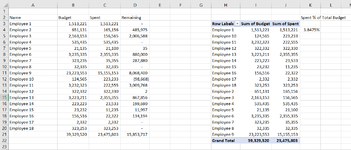
I am trying to produce a pivot table off of data that would show what % of a grand total budget that has been spent on an individual employee.
In the example below, I have a list of employees, their budget, how much of the budget is spent and how much remains. The pivot table should update dynamically as values in the data change, and in column K I would like to have the pivot reflect the fact that Employee 1, at ~1.5M accounts for 3.84% of the total budget spend, as I've indicated with a formula outside of the Pivot. I'd like it to be a calculated pivot field so it automatically updates as the data changes.
| Book1 | ||||||||||||||||
|---|---|---|---|---|---|---|---|---|---|---|---|---|---|---|---|---|
| A | B | C | D | E | F | G | H | I | J | K | L | M | N | |||
| 1 | ||||||||||||||||
| 2 | Name | Budget | Spent | Remaining | Spent % of Total Budget | |||||||||||
| 3 | Employee 1 | 1,513,221 | 1,513,221 | - | Row Labels | Sum of Budget | Sum of Spent | |||||||||
| 4 | Employee 2 | 651,131 | 165,156 | 485,975 | Employee 1 | 1,513,221 | 1,513,221 | 3.8475% | ||||||||
| 5 | Employee 3 | 2,163,153 | 156,565 | 2,006,588 | Employee 10 | 124,565 | 223,233 | |||||||||
| 6 | Employee 4 | 535,435 | 535,435 | - | Employee 11 | 3,232,323 | 222,555 | |||||||||
| 7 | Employee 5 | 21,135 | 21,100 | 35 | Employee 12 | 322,332 | 322,330 | |||||||||
| 8 | Employee 6 | 3,235,335 | 2,355,335 | 880,000 | Employee 13 | 3,223,211 | 2,355,355 | |||||||||
| 9 | Employee 7 | 323,235 | 35,355 | 287,880 | Employee 14 | 223,223 | 23,533 | |||||||||
| 10 | Employee 8 | 32,335 | 32,335 | - | Employee 15 | 23,232 | 11,235 | |||||||||
| 11 | Employee 9 | 23,223,553 | 15,155,153 | 8,068,400 | Employee 16 | 156,516 | 22,322 | |||||||||
| 12 | Employee 10 | 124,565 | 223,233 | (98,668) | Employee 17 | 2,332 | 2,332 | |||||||||
| 13 | Employee 11 | 3,232,323 | 222,555 | 3,009,768 | Employee 18 | 323,253 | 323,253 | |||||||||
| 14 | Employee 12 | 322,332 | 322,330 | 2 | Employee 2 | 651,131 | 165,156 | |||||||||
| 15 | Employee 13 | 3,223,211 | 2,355,355 | 867,856 | Employee 3 | 2,163,153 | 156,565 | |||||||||
| 16 | Employee 14 | 223,223 | 23,533 | 199,690 | Employee 4 | 535,435 | 535,435 | |||||||||
| 17 | Employee 15 | 23,232 | 11,235 | 11,997 | Employee 5 | 21,135 | 21,100 | |||||||||
| 18 | Employee 16 | 156,516 | 22,322 | 134,194 | Employee 6 | 3,235,335 | 2,355,335 | |||||||||
| 19 | Employee 17 | 2,332 | 2,332 | - | Employee 7 | 323,235 | 35,355 | |||||||||
| 20 | Employee 18 | 323,253 | 323,253 | - | Employee 8 | 32,335 | 32,335 | |||||||||
| 21 | 39,329,520 | 23,475,803 | 15,853,717 | Employee 9 | 23,223,553 | 15,155,153 | ||||||||||
| 22 | Grand Total | 39,329,520 | 23,475,803 | |||||||||||||
| 23 | ||||||||||||||||
| 24 | ||||||||||||||||
| 25 | ||||||||||||||||
| 26 | ||||||||||||||||
Sheet1 | ||||||||||||||||
| Cell Formulas | ||
|---|---|---|
| Range | Formula | |
| K4 | K4 | =GETPIVOTDATA("[Measures].[Sum of Spent]",$H$3,"[Range].[Name]","[Range].[Name].&[Employee 1]")/GETPIVOTDATA("[Measures].[Sum of Budget]",$H$3) |
| D3:D20 | D3 | =B3-C3 |
| B21:D21 | B21 | =SUM(B3:B20) |