Excel Power Pivot with 2 measures in Value column

[raysooch]

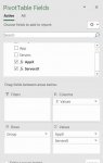
I have an excel Power Pivot, using measures. Here is what the current output looks like. The server column is the result of a measure using a concatenatex function:

Note that the Servers exist within a Group, and that each App defined in a Group are all on the same set of Servers. To avoid the duplicate information, I would like the result to look like this:

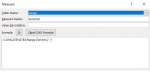
My thought is to have 2 measures, both in the value column of the pivot table and use the appropriate DAX formulae to create the desired result. One measure would determine the Apps within a group; the other measure would determine the Servers within that same group, for the set of Apps. Is there a way to do this?

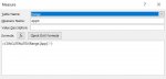
I need a way to redo my Power Pivot to match the second example.

 

[alansidman]

In PP, I built two measures using the DAX formula ConcatenateX. See images below.

Book1
	A	B	C
3	Group	AppX	ServersX
4	Group A	App1	sv1, sv2, sv3, sv4, sv5
5	Group B	App4	sv6, sv7
6	Group C	App5	sv8, sv9, sv10, sv11
Sheet2

EDIT: Just noticed that I got the servers right but not the Apps. Will try again and post when I get a result.

 

[alansidman]

What does your raw data look like before you built the PT. That may help me to get the Apps correct.

 

[raysooch]

@alansidman, your solution was PERFECT! My original data looks like this:

And the pivot out looks like this:

I even managed to figure out how to do line returns on the Appx column. You have saved my day!! Thanks so much.

Ray

 

[alansidman]

Thanks for the feedback. Glad you got what you needed.

 

[raysooch]

Okay, I have another related question. I have expanded my original data source to add a new column, DC. Each app lives on a different set of servers, in each DC. Here is a snippet of the updated data source:

Note the result:

However, by definition of this data set, all apps exist in both DCs, just on a different set of servers within a given DC...so the Appx column is duplicate for each subsequent DC. In this example, I only have 2 DCs, but the real data has more, so the duplicate columns just continue. Is there a way to write the pivot so that the dupe column is only presented once, and not duplicated for each DC? I desire the final output to look like this:

Thanks!
Ray

 

[raysooch]

Regarding the last inquiry to remove the duplicate column (because of the filter with selected DC values), I think I found a solution. I discovered the concept of "sets" in pivot tables. In a pivot table, click on Fields, Items & Sets, and then click in Create Set Based on Column Items. You will have to have filtered your original pivot on whatever filter was used, in my case the DC filter. Then within the SET, you can delete the columns that you do not desire; in my case, it was all of the Appx columns, except the first one. The other positive side affect is that I could create a separate set for each group that I was previously filtering on (DC in this case), such that in the future, when I wish to see the data within a set, just click on the specified set and the pivot table is displayed, for the filter defined within the set. A hidden gem in the complex world of Excel Power Pivot!