-
If you would like to post, please check out the MrExcel Message Board FAQ and register here. If you forgot your password, you can reset your password.
You are using an out of date browser. It may not display this or other websites correctly.
You should upgrade or use an alternative browser.
You should upgrade or use an alternative browser.
Excel VBA - color/shade alternating rows in filtered list
- Thread starter robertvdb
- Start date
Excel Facts
What do {} around a formula in the formula bar mean?
{Formula} means the formula was entered using Ctrl+Shift+Enter signifying an old-style array formula.
VBA Code:
Sub vv()
With Intersect(Range("A1:A" & Cells(Rows.Count, 1).End(3).Row).EntireRow, ActiveSheet.UsedRange)
    .FormatConditions.Delete
    .FormatConditions.Add Type:=xlExpression, Formula1:="=MOD(SUBTOTAL(3,$A$1:$A1),2)=0"
    .FormatConditions(1).Interior.ColorIndex = 37
End With
End Sub
Above assumes there are no blank cells in column A.
Upvote
0
Solution
Thanks footoo but this will not work, since the row numbers are not a natural serie 1,2,3,4,5 etc.
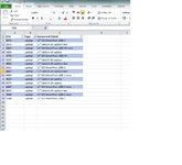
What I need is kind of a loop which starts at the first row, then shades this first row, then shades the row 2 lines below, etc until the last row.
What I need is kind of a loop which starts at the first row, then shades this first row, then shades the row 2 lines below, etc until the last row.
Upvote
0
The row numbers are irrelevant.Thanks footoo but this will not work, since the row numbers are not a natural serie 1,2,3,4,5 etc.
The only caveat : there must be no blanks in column A.
Why don't you try it?
Upvote
0
That is what the code does based on column A.All I still want to do is to better define the range --> from the top row until the last row.
Is there a problem?
If the code is based on a loop, it would probably be quite slow :
VBA Code:
Sub v()
Dim rng As Range, lc&, x&, cel As Range
Set rng = Range("A2:A" & Cells(Rows.Count, 1).End(3).Row).SpecialCells(xlCellTypeVisible)
Cells.Interior.ColorIndex = xlNone
lc = Cells(1, Columns.Count).End(xlToLeft).Column
x = 1
For Each cel In rng
    If x Mod 2 = 0 Then Range(cel, Cells(cel.Row, lc)).Interior.ColorIndex = 37
    x = x + 1
Next
End Sub
Upvote
0
Similar threads
- Replies
- 4
- Views
- 152
- Question
- Replies
- 10
- Views
- 963
- Solved
- Replies
- 6
- Views
- 247


