Excel VBA If Then Copy Paste Format

[SandyBeach]

I have a range which contains individual cell formatting which makes up specific designs. The range is quite large - 500 columns x 300 rows - and is trimmed as required by a VBA routine in order for the design to fit specific dimensions. Trimming is not just by cutting off the surplus right hand columns or bottom rows as the trimming modifies both the size and elements of the design. So, trimming may be effected by cutting off both left and right hand columns, or just the left hand columns, or just the top rows, etc. That is stage 1 and it works well.

Stage 2 requires the trimmed design/range - for which I know the exact number of columns and rows (which could be 500 x 300 but is generally not) - to be copied to another range of exactly the same size and which contains other design elements. Given the design is all formats I want to be able to look at each destination cell to determine if it is occupied (probably by an integer) before copying and pasting from the original range. So, the routine needs to look at, say, the top left hand cell of the destination range and identify if it it is vacant or filled before copying the format in the top left cell of the source range. If the destination cell is vacant, the contents are copied and pasted. If the destination cell is occupied, the routine moves on without copying and pasting.

I have fiddled about with some code but it is so bad i am not going to present it here!

All suggestions gratefully received.

 

[aRandomHelper]

Welcome to the forum!

So, the routine needs to look at, say, the top left hand cell of the destination range and identify if it it is vacant or filled

Only the top left cell needs to be checked? and not any other cells of the 500x300 range?

How do you identify if it's vacant or filled? cell value? cell colour? or?

I have fiddled about with some code but it is so bad i am not going to present it here!

Showing roughly some code even if it doesn't work can help others understand what you're trying to do. You could be copying from sheet 1 of workbook A to sheet 3 of workbook B -- details like that if not mentioned could be picked up from the code.

 

[SandyBeach]

Thank you for your response. Some background may help. A long time ago I was a very competent Fortran user. I followed that into IFPS (a financial language with Fortran and Basic as the foundation) and used that for 10+ years. Then PCs, Lotus, QuattroPro and finally Excel came on the scene. My work focus was always on projects for which specific (one design) models were developed, ie there were few actions which benefited from automation other than print, reset to default values etc. With advent of spreadsheets my life became easier. I managed the few repetitive activities with basic macros. My point is over the years I found I could manage everything I needed through the function line, ie I did not need VB. So my VB skills are poor - and gained mostly by hunting down code that works on the internet. This time, nothing I tried worked. As a result i deleted every attempt in disgust so I have nothing to show.

Let's say the 500 x 300 range (C x R) range has been trimmed to 52 x 32 (C x R) with the top left point being located at I34, ie the range is I34:BH65. I want to copy the format in every cell in that range to a new range of identical size in a new location - eg a new worksheet, preferably with the top left point at I34 - BUT ONLY IF there is nothing in the applicable destination cell. So, if we select I34 (Worksheet1) and copy it to I34 (Worksheet2), only paste the format from I34 (Worksheet1) if there is nothing in I34 (Worksheet2). As noted previously, if I don't want a format pasted to a particular cell then I will put a positive number in the destination cell, so the test can be if I34 (Worksheet2) =0, paste; if I34 (Worksheet2) >0, don't paste.

Do that for every cell in the range, in this case 1,664 cells (with the max being 150,000 cells).

 

[aRandomHelper]

Thanks for providing some explanation.

More questions:

the range is I34:BH65. I want to copy the format in every cell in that range to a new range of identical size in a new location - eg a new worksheet, preferably with the top left point at I34

I understand you mentioned the check to be 1 cell at a time, then do the copy/paste if the destination cell is vacant (value = 0). What happens if any of the destination cells are occupied? Are only those cells ignored, or should the whole process be stopped?

only paste the format

So like Paste Special -> Formats?

Let's say the 500 x 300 range (C x R) range has been trimmed to 52 x 32

You mentioned this is being trimmed by another macro earlier, which works fine. After that, how do you know that the range of 52 x 32 is actually range I34:BH65 ? Do you select the cells manually, or are you expecting the macro to find this range itself based on some criteria?

 

[SandyBeach]

If a destination cell is occupied the paste does not occur and the process moves to the next cell. This continues until the range I34:BH65 (or whatever) on Sheet1 has been interrogated. Then the process stops.

You mentioned Paste Special. When I was working out what I wanted to do manually I just used Copy and Paste. That seemed to bring the formatting over to the destination cell.

Aah, this is interesting. One way of doing it is to have a blank (ie no design) 500 x 300 range waiting at I34 on Sheet2 and then run the trimming routine with the same input commands. That will give me an identical 52 x 32 range (or whatever) to which I will add the additional components - around which I want the design from Sheet1 to be pasted.

At this stage I am using a simple "in cell" (if that is the right term) test to decide whether the additional pattern should be created. All the "If Then Else" formulae in 150,000 cells bulks up the workbook but I can make it work - and I know it will be trimmed later. A VBA alternative would be nice but its a distant second at the moment.

 

[aRandomHelper]

If it's not too inconvenient, can you share the macro that is doing the trimming?

I am still trying to understand how do you "select" or "choose" the 52 x 32 (for example) cells to be copied after running the trimming macro.
Do you do it visually, and just highlight (select) the 52 x 32 cells, then you want to run this second macro that does the copying over to sheet 2?

What I am trying to achieve is to, as much as possible, make the macro dynamic. We can of course hard-code the cells (I34:BH65) into the macro but it wouldn't make sense if this range is different every time, which it most likely would be.

So let me try to picture your work process:
1) You start off with a blank sheet of 500 x 300 cells
2) You do some design changes (I assume entering some values and formatting here and there, or with formulas into parts of the 500x300 range)
3) You run macro-A which does the trimming of cells, down to the area with the "design" ?
4) You check sheet 2 for the similar trimmed area and plot whichever cells you do not want the "design" being copied over with a "1"
5) You want to run macro-B which now do the copying of the trimmed range from sheet 1 to sheet 2, ignoring cells with a "1" in sheet 2

Is my understanding correct?

 

[SandyBeach]

Your points 1 to 3.
I have a bunch of designs set up in 500 x 300 ranges with the top left cell at I34 (I have input parameters in the other left hand columns).
I select a design and run the trimming macro to present it the way required and to fit the desired size.
The trimming routine is actually two macros - I run the column trim first and then the row trim. (Hopefully I will be able to show them below). There is no reason for them to be separate other than for visual checking after the column trim.

Your point 4 - yes
Your point 5 - yes

...and it all seemed so simple when I started. Thank you for your interest.

Macros
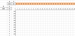
The macros refer to ranges which contain either X or Y. The X or Y is determined by "in cell" calculations fed by the assumptions found in columns A to H. So below, 450 in the X box means 450 columns are to be deleted and 50 saved; Same logic for the columns.

Sub DeleteColumns()

Dim rng As Range
Dim i As Integer, counter As Integer

'Set the range to evaluate to rng.
Set rng = Range("i31:sn31")

'initialize i to 1
i = 1

'Loop for a count of 1 to the number of columns
'in the range that you want to evaluate.
For counter = 1 To rng.Columns.Count

'If cell i in the range contains an "x",
'delete the column.
'Else increment i
If rng.Cells(i) = "X" Then
rng.Cells(i).EntireColumn.Delete
Else
i = i + 1
End If

Next

End Sub

Sub DeleteRows()

Dim rng As Range
Dim i As Integer, counter As Integer

'Set the range to evaluate to rng.
Set rng = Range("g34:g333")

'initialize i to 1
i = 1

'Loop for a count of 1 to the number of rows
'in the range that you want to evaluate.
For counter = 1 To rng.Rows.Count

'If cell i in the range contains an "x",
'delete the row.
'Else increment i
If rng.Cells(i) = "X" Then
rng.Cells(i).EntireRow.Delete
Else
i = i + 1
End If

Next

End Sub

 

[aRandomHelper]

The X or Y is determined by "in cell" calculations fed by the assumptions found in columns A to H. So below, 450 in the X box means 450 columns are to be deleted and 50 saved; Same logic for the columns.

Alright, so it became much clearer now. From the macros, I can see that the entire row or column would be deleted when "X" is found in any of the corresponding row/column.

What happens after that running both of those macros? are cells G31:H31 and F33:G33 being cleared off? If yes, what do those formulas in ranges i31:sn31 and g34:g333 show after the deletion?

 

[SandyBeach]

This is what it looks like before and after being run:

52 is in cell H31
32 is in cell G33

Formula for I31 and G34..

I31 formula runs to BH31 because all other columns have been deleted.
G34 formula runs to G65. because all other rows have been deleted.

 

[aRandomHelper]

Can you try running this?
Please try on a copy of the workbook first.

Remember to change the "Sheet7" and "Sheet11" to your "sheet1"/"sheet2" accordingly, I am not sure what are the sheet names.

Sub SandyBeach()
    Dim ws1 As Worksheet, ws2 As Worksheet
    Dim r As Range, c As Range
    
    Set ws1 = Sheets("Sheet7") '<-- "From sheet": change sheet name accordingly
    Set ws2 = Sheets("Sheet11") '<-- "To sheet": change sheet name accordingly
    
    Application.ScreenUpdating = False
    With ws1
        Set r = .Range("I34").Resize(.Range("G33").Value, .Range("H31").Value)
    End With
    
    With ws2
        For Each c In r
            If .Range(c.Address(0, 0)).Value <> 1 Then
                c.Copy .Range(c.Address(0, 0))
            End If
        Next
    End With
    Application.ScreenUpdating = True
    
End Sub