Excel VBA - Loop Through Worksheet, Copy Cells, Paste into New Worksheet

sdgz747

New Member
Joined
Feb 2, 2021
Messages
9
Office Version
  1. 2016
Platform
  1. Windows
Hello, I am new to VBA and my knowledge is limited. I will try my best to provide an accurate description, but if additional clarification is needed please reach out. I am trying to create a VBA to accomplish the following:
  1. I need to replicate a Master worksheet based on the number of rows from an Import worksheet
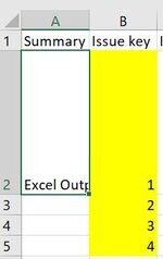
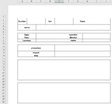
    1. Master worksheet: Master.JPG
    2. Import worksheet:Import.JPG
      1. In the example above, I would expect to see 4 new worksheets be created. Additionally, with the code I have so far, the new tabs will be named 1, 2, 3, and 4
  2. I also need to fill in the cells in the created worksheets with the associated data pulled in from the Import worksheet row
    1. I believe I need some sort of loop to pull in data from each row from the Import worksheet until I reach the end of the worksheet
    2. Identified rows from the Import worksheet I need to copy are (keep in mind, I need to start from row 2 then proceed until there are no more rows with data):
      1. A, B, O, Q, Y, BG, BW, CB, CC, CD, CE, CH, CJ
    3. Identified rows I need to paste in the newly created worksheets are (the rows will always be the same, but the worksheet will always be new):
      1. B7:C8, E7:F8, I7:J8, C14:E14, C15:E15, C16:E16, H14:J14, H16:J16, E20:J21, E22:J22, E23:J23, A27:J33, A37:J43
  3. This may be overkill, but is there some kind of check I can run to ensure duplicates do not occur?
The code I have so far replicates the Master worksheet until there is no more data in the Import worksheet. In the example I've given, 4 new worksheets will be created using the Master worksheet template and the worksheet names will be 1, 2, 3, and 4. I have not yet been able to figure out the looping required to pull in data. The code is as follows:

VBA Code:
Sub makeTPRs()

' Declare variables sh1, sh2, c
Dim sh1 As Worksheet
Dim sh2 As Worksheet
Dim c As Range

' Set sh1 to TPR_Master worksheet
Set sh1 = Sheets("TPR_Master")
' Set sh2 to Jira_Import worksheet
Set sh2 = Sheets("Jira_Import")

' Count each number of filled rows in column 2, for every row counted create a new worksheet
' based on the TPR_Master worksheet and give the tab the associated TPR value
    For Each c In sh2.Range("B2", sh2.Cells(Rows.Count, 2).End(xlUp))
        sh1.Copy Before:=sh1
        ActiveSheet.Name = c.Value
    Next

End Sub
 

Excel Facts

Using Function Arguments with nested formulas
If writing INDEX in Func. Arguments, type MATCH(. Use the mouse to click inside MATCH in the formula bar. Dialog switches to MATCH.
The copy and paste rules for Excel are the same whether doing it manually or with code. The paste range has to be able to accomodate the copy range. The description in the OP does not appear to comply with that rule, even after figuring out that it is columns and not rows that are defined for the copy range. Maybe you want to read what you wrote as though you don't yhave the worksheet in front of you and give us a better description of the copy and paste ranges. Bear in mind that you cannot copy a single row or single column of data and then try to paste it into a two dimensional range, nor vice versa. Also, the images posted appear to have several merged cells. VBA is not happy when working with merged cells and often generates error messages or procuces undesired results. If any of the copy and paste ranges are merged, they need to be unmerged to run code efficiently.
 
Last edited:
Upvote 0
Hello @JLGWhiz, thank you for your response. Here is what I'm trying to do and hopefully this will help clarify things. I want to take an export of data, create multiple tabs from a master sheet based on the number of rows from the export (i.e., if there are four rows in the export data sheet, I would expect 4 new tabs to be created), and fill in cells in the new sheets based on the exported data. The data in each row from the export is unique, the selected data must remain unique (hence the need for creating multiple tabs). Please let me know if I can clarify further.

As a side note, the code I have provided creates new tabs. The code replicates the Master Sheet and uniquely names the worksheet based on data within a column from the export data.

I will also fix the master sheet so it is no longer set up with merged cells.
 
Upvote 0
That part was understood, but it does not address the copy and paste issue. You cannot copy and paste as described in the OP. A better explanation of the ranges to copy and the paste destination is needed. The current exp;lanation appears to be impractical since it would likely generate error messages.

  1. Identified rows from the Import worksheet I need to copy are (keep in mind, I need to start from row 2 then proceed until there are no more rows with data):
    1. A, B, O, Q, Y, BG, BW, CB, CC, CD, CE, CH, CJ <<<These are columns
  2. Identified rows I need to paste in the newly created worksheets are (the rows will always be the same, but the worksheet will always be new):
    1. B7:C8, E7:F8, I7:J8, C14:E14, C15:E15, C16:E16, H14:J14, H16:J16, E20:J21, E22:J22, E23:J23, A27:J33, A37:J43 <<<These are ranges
You also need to clarify the merged cell issue. If you are trying to copy or paste where there are merged cells, that can also present problems with vba.
 
Last edited:
Upvote 0
Okay, I'm tracking now @JLGWhiz. I guess I misunderstood what you were asking. Here's some clarification on the copy / paste:
  • The merged cells in the Master worksheet have been fixed; they are now single cells instead of a merged range. IF there is some way to keep the cells merged that would be helpful. Otherwise, I'll have to figure out a way to workaround it.
  • Copy: copy from the Import worksheet; each row is unique and the identified cells in the row must be pasted into a new tab worksheet keeping the unique information grouped together.
    1. Identified rows from the Import worksheet I need to copy are (keep in mind, I need to start from row 2 then proceed until there are no more rows with data):
    2. A, B, O, Q, Y, BG, BW, CB, CC, CD, CE, CH, CJ
  • Paste: paste into the newly create worksheet; every identified cell in the worksheet is the same, but the worksheet will be unique/new
  • Example: the following is an example of the mapping I'm trying to accomplish
    • Notice, when New Worksheet 2 begins copying the data from the next row occurs; this will repeat until no more rows with data exist
Copy​
Paste​
New Worksheet​
A2C6New Worksheet 1
B2C7New Worksheet 1
BW2C8New Worksheet 1
CB2C9New Worksheet 1
Q2C12New Worksheet 1
Q2C13New Worksheet 1
BG2C14New Worksheet 1
O2H12New Worksheet 1
CC2H14New Worksheet 1
CH2C17New Worksheet 1
CE2C18New Worksheet 1
CJ2C19New Worksheet 1
Y2A22New Worksheet 1
CD2A31New Worksheet 1
A3C6New Worksheet 2
B3C7New Worksheet 2
BW3C8New Worksheet 2
CB3C9New Worksheet 2
Q3C12New Worksheet 2
Q3C13New Worksheet 2
BG3C14New Worksheet 2
O3H12New Worksheet 2
CC3H14New Worksheet 2
CH3C17New Worksheet 2
CE3C18New Worksheet 2
CJ3C19New Worksheet 2
Y3A22New Worksheet 2
CD3A31
New Worksheet 2​
 
Upvote 0
  1. Identified rows from the Import worksheet I need to copy are (keep in mind, I need to start from row 2 then proceed until there are no more rows with data):
  2. A, B, O, Q, Y, BG, BW, CB, CC, CD, CE, CH, C
Please ignore bullet point 1 and 2 in the post above; unfortunately I'm unable to edit my post. :(
 
Upvote 0
I will see if I can work something out with this. If so, I will post back to this thread.
 
Upvote 0
Thank you!

I was thinking a nested loop could work, but I haven't had any success with it. I've looked at different VBA code examples, but I haven't had any success with incorporating it.
 
Upvote 0
See if this is close to what you want.

VBA Code:
Sub t()
Dim ary1 As Variant, ary2 As Variant, sh1 As Worksheet, sh2 As Worksheet, c As Range, i As Long
ary1 = Array("A", "B", "BW", "CB", "Q", "BG", "O", "CC", "CH", "CE", "CJ", "Y", "CD")
ary2 = Array("C6", "C7", "C8", "C9", "C12:C13", "C14", "H12", "H14", "C17", "C18", "C19", "A22", "A31")
Set sh1 = Sheets("TPR_Master")
Set sh2 = Sheets("Jira_Import")
    For Each c In sh2.Range("B2", sh2.Cells(Rows.Count, 2).End(xlUp))
        If c <> "" Then
            For i = LBound(ary1) To UBound(ary1)
                sh1.Range(ary2(i)) = sh2.Cells(c.Row, ary1(i)).Value
            Next
            sh1.Copy After:=Sheets(Sheets.Count)
            Sheets(Sheets.Count).Name = c.Value
        End If
    Next
End Sub
 
Upvote 0
@JLGWhiz, thank you! So far this is working out great. I tweaked it a bit to make a bit more sense for me. I also added a clear master spreadsheet line so it gets cleared up at the end. Here's the code I tweaked:

VBA Code:
Sub t()

Dim ary1 As Variant
Dim ary2 As Variant
Dim sh1 As Worksheet
Dim sh2 As Worksheet
Dim c As Range
Dim i As Long

ary1 = Array("A", "B", "BW", "CB", "Q", "Q", "BG", "O", "CC", "CH", "CE", "CJ", "Y", "CD")
ary2 = Array("C6", "C7", "C8", "C9", "C12", "C13", "C14", "H12", "H14", "C17", "C18", "C19", "A22", "A31")

clrrng = ("C6:J9, C12:E14, H12:J12, H14:J14, C17:J19, A22:J28, A31:J37")

Set sh1 = Sheets("TPR_Master")
Set sh2 = Sheets("Jira_Import")
    
    For Each c In sh2.Range("B2", sh2.Cells(Rows.Count, 2).End(xlUp))
        If c <> "" Then
            For i = LBound(ary1) To UBound(ary1)
                sh1.Range(ary2(i)) = sh2.Cells(c.Row, ary1(i)).Value
            Next
            
            sh1.Copy After:=Sheets(Sheets.Count)
            Sheets(Sheets.Count).Name = c.Value
                    
        End If
        
    Next
    
sh1.Range(clrrng).ClearContents

End Sub
 
Upvote 0

Forum statistics

Threads
1,214,965
Messages
6,122,495
Members
449,088
Latest member
Melvetica

We've detected that you are using an adblocker.

We have a great community of people providing Excel help here, but the hosting costs are enormous. You can help keep this site running by allowing ads on MrExcel.com.
Allow Ads at MrExcel

Which adblocker are you using?

Disable AdBlock

Follow these easy steps to disable AdBlock

1)Click on the icon in the browser’s toolbar.
2)Click on the icon in the browser’s toolbar.
2)Click on the "Pause on this site" option.
Go back

Disable AdBlock Plus

Follow these easy steps to disable AdBlock Plus

1)Click on the icon in the browser’s toolbar.
2)Click on the toggle to disable it for "mrexcel.com".
Go back

Disable uBlock Origin

Follow these easy steps to disable uBlock Origin

1)Click on the icon in the browser’s toolbar.
2)Click on the "Power" button.
3)Click on the "Refresh" button.
Go back

Disable uBlock

Follow these easy steps to disable uBlock

1)Click on the icon in the browser’s toolbar.
2)Click on the "Power" button.
3)Click on the "Refresh" button.
Go back
Back
Top