Excel Vlookup formula to get a Required Details

[Shazir]

I have been using a sheet where i am stuck to do the necessary requirements.

I am trying to get a single employee review in the given table that how many times his review has been done in a year, two or three and so on. If I remove the year then his all review should appear in the above table.

I have been tried with vlookup but its not working.

any help will be highly appreciated

DataSheet

 

[PankajMaheshwari]

Hi @Shazir , please follow this thread nth value.

 

[navic]

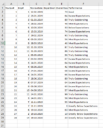
You should have given the expected results (example)
If I understood you well, try the following:

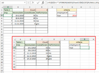
Set the following formulas on Sheet2

In the 'D1' cell copy formula below (change range if you need)

=COUNT(A3:A9)

In the 'A3' cell copy ARRAY formula below (formula finished with CSE, copy down)

=IF($G$3<>"",IFERROR(INDEX(Sheet1!$B$2:$F$29,SMALL(IF((Sheet1!$B$2:$B$29=$G$2)*(--(YEAR(Sheet1!$C$2:$C$29)=$G$3)),ROW(Sheet1!$B$2:$B$29)),ROW($A1:$G1))-1,COLUMN(A1)),""),IFERROR(INDEX(Sheet1!$B$2:$F$29,SMALL(IF(Sheet1!$B$2:$B$29=$G$2,ROW(Sheet1!$B$2:$B$29)),ROW($A1:$G1))-1,COLUMN(A1)),""))

Copy formula to 'B' column and down or
In the 'B3' cell copy ARRAY formula below (formula finished with CSE, copy down)

=IF($G$3<>"",IFERROR(INDEX(Sheet1!$B$2:$F$29,SMALL(IF((Sheet1!$B$2:$B$29=$G$2)*(--(YEAR(Sheet1!$C$2:$C$29)=$G$3)),ROW(Sheet1!$B$2:$B$29)),ROW($A1:$G1))-1,COLUMN(B1)),""),IFERROR(INDEX(Sheet1!$B$2:$F$29,SMALL(IF(Sheet1!$B$2:$B$29=$G$2,ROW(Sheet1!$B$2:$B$29)),ROW($A1:$G1))-1,COLUMN(B1)),""))

In the 'C3' cell copy ARRAY formula below (formula finished with CSE, copy down)

=IF($G$3<>"",IFERROR(INDEX(Sheet1!$B$2:$F$29,SMALL(IF((Sheet1!$B$2:$B$29=$G$2)*(--(YEAR(Sheet1!$C$2:$C$29)=$G$3)),ROW(Sheet1!$B$2:$B$29)),ROW($A1:$G1))-1,COLUMN(D1)),""),IFERROR(INDEX(Sheet1!$B$2:$F$29,SMALL(IF(Sheet1!$B$2:$B$29=$G$2,ROW(Sheet1!$B$2:$B$29)),ROW($A1:$G1))-1,COLUMN(D1)),""))

Copy formula to 'D' column and down or
In the 'D3' cell copy ARRAY formula below (formula finished with CSE, copy down)

=IF($G$3<>"",IFERROR(INDEX(Sheet1!$B$2:$F$29,SMALL(IF((Sheet1!$B$2:$B$29=$G$2)*(--(YEAR(Sheet1!$C$2:$C$29)=$G$3)),ROW(Sheet1!$B$2:$B$29)),ROW($A1:$G1))-1,COLUMN(E1)),""),IFERROR(INDEX(Sheet1!$B$2:$F$29,SMALL(IF(Sheet1!$B$2:$B$29=$G$2,ROW(Sheet1!$B$2:$B$29)),ROW($A1:$G1))-1,COLUMN(E1)),""))

The nested COLUMN function indicates the column number.

The formula works as follows.
The base formula is an IF function consisting of two ARRAY formulas
TRUE argument - Array Formula that returns results if two criteria are active (year and number of clients)
FALSE argument - Array Formula that returns the result if one criterion is active (ie number of clients)

 

[Shazir]

navic​

You are great thank you so much.