Hi,
first time posting here so hopefully this is the right area.")
Please see the attached pictures with sample data. What I need to do is the following:
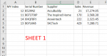
1) only paste data into the first sheet (formatted as already shown in there) and Excel extract data from Sheet 1 to fill in Sheet 2 and Sheet 3
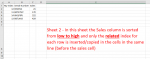
2) Sheet 2 contains only 3 of the 5 columns of Sheet 1: MyIndex, Serial Number and Sales. It is sorted by Sales LOW to HIGH. And next to each Sales cell it has the related Serial Number and MyIndex value.
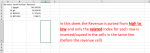
3) Sheet 3 is the same as Sheet 2 (explained in point 2 above) but: 1) instead of Sales it contains the Revenue column and 2) the Revenue Column is sorted from HIGH to LOW
NOTE: If it helps I can make sure that the data pasted on Sheet 1 is always a known/fixed number of rows
If possible:
- not using extra columns/sheets (but if cannot be avoided then that's ok)
- to do it with formulas and not macros/programming
Many thanks
first time posting here so hopefully this is the right area.
Please see the attached pictures with sample data. What I need to do is the following:
1) only paste data into the first sheet (formatted as already shown in there) and Excel extract data from Sheet 1 to fill in Sheet 2 and Sheet 3
2) Sheet 2 contains only 3 of the 5 columns of Sheet 1: MyIndex, Serial Number and Sales. It is sorted by Sales LOW to HIGH. And next to each Sales cell it has the related Serial Number and MyIndex value.
3) Sheet 3 is the same as Sheet 2 (explained in point 2 above) but: 1) instead of Sales it contains the Revenue column and 2) the Revenue Column is sorted from HIGH to LOW
NOTE: If it helps I can make sure that the data pasted on Sheet 1 is always a known/fixed number of rows
If possible:
- not using extra columns/sheets (but if cannot be avoided then that's ok)
- to do it with formulas and not macros/programming
Many thanks