Extracting values from equations shown a chart.

steve case

Well-known Member
Joined
Apr 10, 2002
Messages
823
I created a graph from my data, hovered over my data and right clicked
the mouse. A menu appeared with among other things "add a trend line"
Clicking that, another menu "Trendline Options" appears, I selected the
radio button for Polynomial and selected "Order 2" At the bottom of the
menu I selected "[✓] Display equation on chart" And clicked the [Close] button.

The trend line and the following equation appeared on my graph:

y = 0.0117x² + 1.6021x + 6743.2

Are there any Excel functions i.e., =function(known_y's,known_x's) that
will yield any of those three numbers that appear in the shown equation?

Right now I'm copy and pasting the value for X² into the desired cell.
A function to do that would be super!

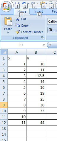
My "X" and "Y" data are in Column "A" and "B" respectively - right on down the sheet.

A function in [C1] =FUNCTION(A:A,B:B) to yield: the 0.0117 for X² is what I'm looking for.

I have Excel 2007
 

Excel Facts

Fastest way to copy a worksheet?
Hold down the Ctrl key while dragging tab for Sheet1 to the right. Excel will make a copy of the worksheet.
There's likely a built-in function for this, but you can do it like so:

Book1
ABCD
1xy9.369450.278717
21100.13654
32110.278717
4312.5
5414
6516
7619
8725
9830
10933
111144
Sheet2
Cell Formulas
RangeFormula
D1D1=INDEX(MMULT(MINVERSE(CHOOSE({1,2,3;2,3,4;3,4,5},10,SUM(A2:A11),SUM(A2:A11^2),SUM(A2:A11^3),SUM(A2:A11^4))),CHOOSE({1;2;3},SUM(B2:B11),SUMPRODUCT(B2:B11,A2:A11),SUMPRODUCT(B2:B11,A2:A11^2))),3)
C1:C3C1=MMULT(MINVERSE(CHOOSE({1,2,3;2,3,4;3,4,5},10,SUM(A2:A11),SUM(A2:A11^2),SUM(A2:A11^3),SUM(A2:A11^4))),CHOOSE({1;2;3},SUM(B2:B11),SUMPRODUCT(B2:B11,A2:A11),SUMPRODUCT(B2:B11,A2:A11^2)))
Press CTRL+SHIFT+ENTER to enter array formulas surrounded with curly braces.
 
Upvote 0
This link:


shows a simpler way:

Book1
ABCDE
1xy0.278717
2110
3211abc
4312.50.2787170.136549.36945
5414
6516
7619
8725
9830
10933
111144
Sheet2
Cell Formulas
RangeFormula
C1C1=LINEST(B2:B11,A2:A11^{1,2},1,0)
C4:E4C4=LINEST(B2:B11,A2:A11^{1,2},1,0)
Press CTRL+SHIFT+ENTER to enter array formulas surrounded with curly braces.


Also much simpler to extend.
 
Upvote 0
There's likely a built-in function for this, but you can do it like so:

Book1
ABCD
1xy9.369450.278717
21100.13654
32110.278717
4312.5
5414
6516
7619
8725
9830
10933
111144
Sheet2
Cell Formulas
RangeFormula
D1D1=INDEX(MMULT(MINVERSE(CHOOSE({1,2,3;2,3,4;3,4,5},10,SUM(A2:A11),SUM(A2:A11^2),SUM(A2:A11^3),SUM(A2:A11^4))),CHOOSE({1;2;3},SUM(B2:B11),SUMPRODUCT(B2:B11,A2:A11),SUMPRODUCT(B2:B11,A2:A11^2))),3)
C1:C3C1=MMULT(MINVERSE(CHOOSE({1,2,3;2,3,4;3,4,5},10,SUM(A2:A11),SUM(A2:A11^2),SUM(A2:A11^3),SUM(A2:A11^4))),CHOOSE({1;2;3},SUM(B2:B11),SUMPRODUCT(B2:B11,A2:A11),SUMPRODUCT(B2:B11,A2:A11^2)))
Press CTRL+SHIFT+ENTER to enter array formulas surrounded with curly braces.

Thanks for the reply

Duplicated your data in columns "A" &"B"

So far I get:
#VALUE!
The note:
Press CTRL+SHIFT+ENTER to enter array formulas surrounded with curly braces.
does not work I held down [CTRL]&[SHIFT] and pressed [ENTER] I assume you remove
the curlies before you try to paste it in there, but I did try it with just because and
removed them and it's still #VALUE!

So I removed the Curlies, and the = sign, pasted the formulas in there and put the
equal signs back in.

There's likely a built-in function for this, but you can do it like so:

I didn't say so in the first post, but I looked through the statistical functions and
some others and didn't find anything that looked like it would work. I tried
=INTERCEPT
to see if it duplicated the linear intercept displayed in the linear equation on the
graph and it didn't, nor did it lead me down any path to find what I'm looking for.

I sure do hope there is like you say like a function for this (-:

I assume the formula in [C1] is copied on down to [C11] in your example

Besides all that, it looks like your formulas have as many terms as there are lines of data.
if that's the case and there's no easy way to generate them then..... I have lots of data
sets to look at and they vary in length with 30 to 100 lines or so of data.
 
Upvote 0
The formulas from post 2 I got from a web site, and they do work, but yes, they are quite long. Let's skip them for now and look at the formulas from post 3. Much simpler. Someone discovered a clever way to use a built-in function.

Open a blank worksheet. Then from my example in post 3, click on the 2-sheet icon between the 1 and the A. It should say "Range copied to clipboard" on the top of the screen. Go to your worksheet, select A1 and click Paste. That should give you the example. This procedure does not preserve the Control+Shift+Enter process, but as it happens, the C1 formula does not require that after all, you should get the right answer.

However, if you look at the C4:E4 values, they are all the same. To get the different coefficients, select C4:E4, press F2, then hold down the Control and Shift keys and press Enter.

Let me know if this works for you.
Thanks Eric, I'll try it in the morning. :)
 
Upvote 0
OK, so now it generated some numbers as opposed to #VALUE!

First off let's see what your sample data generates
when graphed with the show equation option selected:

y = 0.4261x2 - 1.1511x + 11.375

With The LINEST formulas in the cells as follows

[C1] =LINEST(B2:B11,A2:A11^{1,2},1,0)
[C4] =LINEST(B2:B11,A2:A11^{1,2},1,0)

It generates this number:

0.278717407

Which is exactly what your example shows but it doesn't relate to
any of the three terms in the Y= equation above. So I'm confused.

I don't understand what

To get the different coefficients, select C4:E4, press F2,
then hold down the Control and Shift keys and press Enter.

is supposed to do other than put 0.278717407 in cells [C1]-[C4]

What coefficients?
Where are they supposed to go?
What do they do?
What do they have to do with getting the x² value from the data?

I'm mostly a copy and paste guy. I do some macros and formulas
and I tinker with them to fit my needs. So if there's a LINEST
function that produces the 0.4261 from the equation option, as
I have shown above, I will be able to manipulate it to fit varying
amounts of data. At least I'm pretty sure I can (-:

I really do appreciate that you are working on this issue. I've
been coming to Mr. Exel over the years and it has been a great
FREE resource. Helped me keep my job more than a few times. I'm
retired now, but I do have some interests that involve number
crunching of one sort or another.

Stay well, wear your mask when out and about (-:

Best regards
 
Upvote 0
Somehow your inserted graph does not match what I have. This is what I got with the same data:

Untitled.jpg


I followed the procedure you outlined, select the data (A2:B11), insert chart, insert trendline (polynomial order 2), show equation. Then the formula in C4:E4 shows the same coefficients as the equation on the graph. The C1 formula just shows the first one.

I tried tweaking the parameters to see if I could figure out how you got your equation, but I couldn't. I got fairly close by selecting A2:B10, so I'd guess there's something different in the way we made the charts.
 
Upvote 0
The problem is the missing data for [B11] :
image.png


so if I select [A2:B12] Press [F11] to create my graph, select polynomial and show the equation it comes out exact.
So I may have to do some rearranging of data to make this work. One set to create the graph and correct value
for x² and another for LINEST to work and deliver x² as I requested I have this feeling that the blank in [B11] will
trip up LINEST. My data almost always has missing "Y" values. But I'm feeling good about this because running
a second data set with the blanks not shown will be easy to create. I hope to post a success story later today (-:
 
Upvote 0

Forum statistics

Threads
1,214,605
Messages
6,120,473
Members
448,967
Latest member
visheshkotha

We've detected that you are using an adblocker.

We have a great community of people providing Excel help here, but the hosting costs are enormous. You can help keep this site running by allowing ads on MrExcel.com.
Allow Ads at MrExcel

Which adblocker are you using?

Disable AdBlock

Follow these easy steps to disable AdBlock

1)Click on the icon in the browser’s toolbar.
2)Click on the icon in the browser’s toolbar.
2)Click on the "Pause on this site" option.
Go back

Disable AdBlock Plus

Follow these easy steps to disable AdBlock Plus

1)Click on the icon in the browser’s toolbar.
2)Click on the toggle to disable it for "mrexcel.com".
Go back

Disable uBlock Origin

Follow these easy steps to disable uBlock Origin

1)Click on the icon in the browser’s toolbar.
2)Click on the "Power" button.
3)Click on the "Refresh" button.
Go back

Disable uBlock

Follow these easy steps to disable uBlock

1)Click on the icon in the browser’s toolbar.
2)Click on the "Power" button.
3)Click on the "Refresh" button.
Go back
Back
Top