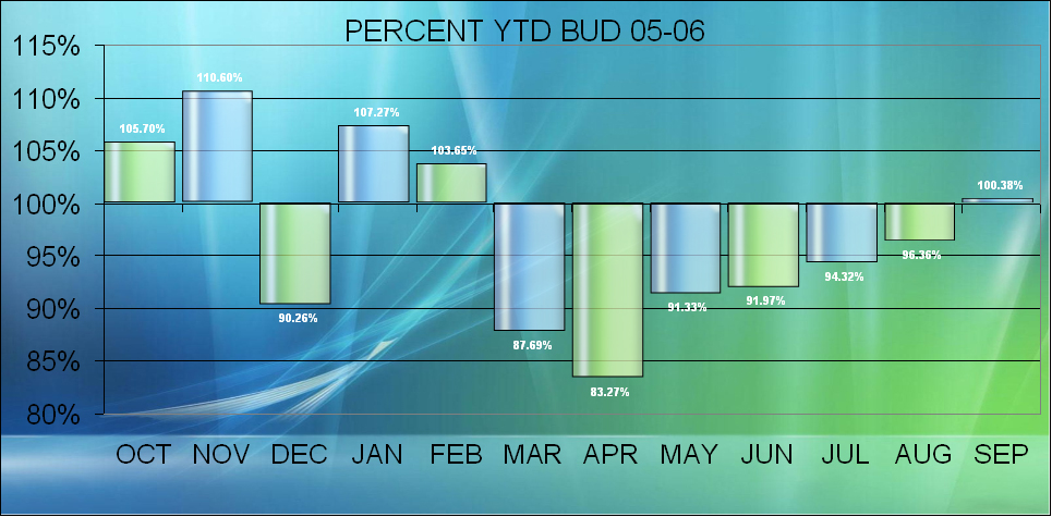
Figured out how to fake transparent 3D bar chart

[babycody]

Hi everyone. I have created a Pivot Table Chart and I want to display a label above each column with the values they represent. The problem is that when I change the month I lose the labels above the columns. I also can't get a custom chart to stay. It always goes back to the built in charts. Is there a way to prevent this from happening? Thanks!

 

[mrhartley]

Hi, I think you might find the only way to do this is to write a macro to put back the setting that you lose.

Regards
~Mark

 

[babycody]

I ended up referencing the pivot table in a regular range using GETPIVOTDATA function, and regular old ="some cell". Then I created a chart from that range. Now everything works normally. Hid the new range under the chart for asthetics. Will probably forget I did that one day, and drive my self bonkers trying to figure out where that range is. Thanks for the opinion mrhartley.

 

[mrhartley]

OMG sorry I forgot thats exactly what I have done in the past, totally forgot about that and your right its easy to forget your new chart is hiding the data lol

Glad your sorted

 

[tusharm]

Several other ways to do this, none of which require duplicating data:

1) Create a chart from a named formula that refers to the PT data. The advantage of this approach is that if the PT shrinks/grows, the chart auto-adjusts.

2) Create an empty chart and then specify the source as the PT data. The key here is to not include any of the PT headers.

2a) Select the empty chart, then Chart | Add Data... and specify the PT cells of interest

2b) Select the empty chart, then Chart | Source Data... | Series tab | specify the X and Y values as required

2c) Select the PT data range, copy, select the chart, and Edit | Paste Special...

2d) Select the PT data range, move the cursor over the edge so that you can drage the range, and drag it on to the chart.

Of all the ways listed in item 2 above, 2b probably gives you the most flexibility -- especially if you have multiple row fields.

I ended up referencing the pivot table in a regular range using GETPIVOTDATA function, and regular old ="some cell". Then I created a chart from that range. Now everything works normally. Hid the new range under the chart for asthetics. Will probably forget I did that one day, and drive my self bonkers trying to figure out where that range is. Thanks for the opinion mrhartley.

 

[babycody]

Thank you tusharm! It's nice to get advice from a real expert on charts like you. I will try all of these ways to familiarize myself with them. Thanks again.

P.S. You wouldn't happen to know how to make transparent 3d bar charts would you? I know how to do the 2D ones, but can't find anything on 3D.

 

[tusharm]

Unfortunately, formatting options with 3D charts are extremely limited, though they *may* improve with 2007.

Thank you tusharm! It's nice to get advice from a real expert on charts like you. I will try all of these ways to familiarize myself with them. Thanks again.

P.S. You wouldn't happen to know how to make transparent 3d bar charts would you? I know how to do the 2D ones, but can't find anything on 3D.

 

[babycody]

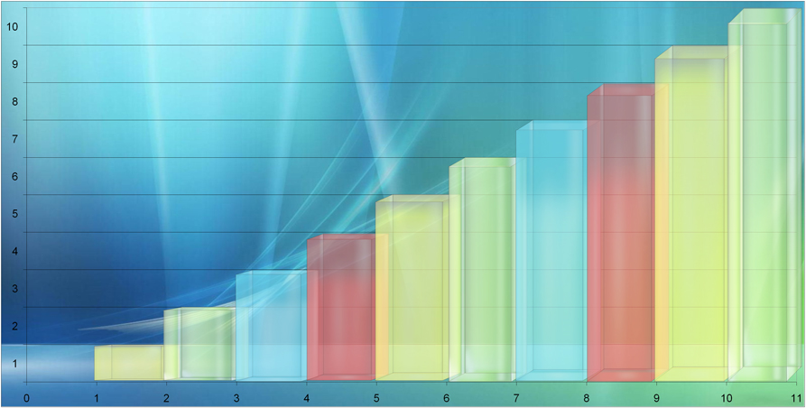
Tusharm managed to make a transparent 3d chart on my own within Excel mostly. What do you think? If anyone would like to know how I did it then post a request here, and I will make a tutorial. These bars probably could have used darker outlines to better define them, but that is doable. The width of the bars needs to be adjusted, and I need to work on the angles too. Remember this was my first attempt so it can be better. You could probably make one of those zig zag arrows you see on charts in a simular fashion. Tusharm notice that these bars unlike Excel's 3d bars line up, at the top, with the lines on the wall. Please critique.

 

[Jon Peltier]

Want my opinion? It's horrible. The special effects completely overwhelm any data in the chart. A simple column or line chart would show the data much more clearly, in a smaller space, with much less distraction from transparent effects and swooshes.

To improve it:

Remove all 3D effects, especially since there's no third variable in the chart.
Remove all nonstandard formatting, such as multicolored backgrounds, transparencies, shadows, swooshes, etc.

 

[babycody]

Thanks Jon for the honest opinion. I was asked to make some eye catching charts for my boss. He didn't like the standard charts including the backgrounds. He said that the charts on this site looked nice: http://www.dotnetcharting.com/gallery/ I will dump the 3D since I respect your opinion on charts. Oh well, the experience taught me a few new tricks. I will probably go with something like this:

Source for technique: http://j-walk.com/ss/excel/usertips/tip071.htm