Fill values from fixed value conditional to time span

[JohnDooe]

Hello,

I can't wrap my head around this. Maybe someone here can help me out.

Context
I need to create an excel spreadsheet to help plan the distribution of welcome packages to club members.
These packages contain shirts which are handmade (take the longest to make of the components). So, to help plan the rest we'd like to know when they are ready. Production speed of the shirts varies (depending on helpers available)

Spreadsheet
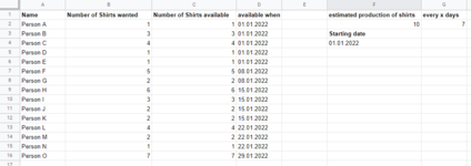
The values in column B are entered manually. Same with F2; F4 and G2.
I would like excel to fill column c and d according to the values in F2; F4 and G2.

Fill column D with the starting date from F4 until we reach the value entered in F2. Then start over and add the value from G2 to F4.
And so on.

To be perfectly honest: I experimented for a few days and spent some time googling but have to admit this is beyond my skills.
Any help would be greatly appreciated.

 

[Marcelo Branco]

Welcome to Mr Excel Forum

Maybe with two helper columns (see columns I and J)

Pasta1
	A	B	C	D	E	F	G	H	I	J
1	Names	Qty wanted	Available when			Qty	Days		Dates	Available
2	Person 1	1	01/01/2022			10	7		01/01/2022	10
3	Person 2	3	01/01/2022						08/01/2022	20
4	Person 3	4	01/01/2022			Start			15/01/2022	30
5	Person 4	1	01/01/2022			01/01/2022			22/01/2022	40
6	Person 5	1	01/01/2022						29/01/2022	50
7	Person 6	5	08/01/2022						05/02/2022	60
8	Person 7	2	08/01/2022						12/02/2022	70
9	Person 8	6	15/01/2022						19/02/2022	80
10	Person 9	3	15/01/2022						26/02/2022	90
11	Person 10	2	15/01/2022						05/03/2022	100
12	Person 11	2	15/01/2022						12/03/2022	110
13	Person 12	4	22/01/2022						19/03/2022	120
14	Person 13	2	22/01/2022						26/03/2022	130
15	Person 14	1	22/01/2022						02/04/2022	140
16	Person 15	7	29/01/2022						09/04/2022	150
17
Plan9

Cell Formulas
Range	Formula
I2:I16	I2	=F$5+(ROWS(I$2:I2)-1)*G$2
J2:J16	J2	=F$2*ROWS(J$2:J2)
C2:C16	C2	=INDEX($I$2:$I$16,IFERROR(MATCH(SUM(B$2:B2),J$2:J$16)+IF(ISNA(MATCH(SUM(B$2:B2),J$2:J$16,0)),1,0),1))

Hope this helps

M.

 

[JohnDooe]

Thank you for your help. Greatly appreciated.

I tried this to transfer this to my spreadsheet and I get #name errors. Even if I try it with the exact same values and positions.

 

[Marcelo Branco]

I get #name errors.

What Excel version are you using?

M.

 

[Marcelo Branco]

The formulas I suggested use functions available since Excel 2007 and later versions.

Looking at your profile, I see Windows and Office 365 - I don't understand why the #NAME error occurred in your case (???)

M.

 

[Fluff]

Are you trying this in Excel, rather than some other App, such as Goggle Sheets?
If you are using xl, what language does your version use?