=FILTER, Review Meeting process

[ozzborn]

I am using Windows 10 and Office 365.

Sheet1 below is the primary data source for Sheet2 breaking out meetings in different allocations of time.

Meetings are only held on Tues, and Wed, and Fridays. Each meeting has 1 to 4 Topics they discus and decide if it needs to go onto the next meeting.

Meetings are placed into the schedule based on the topic. Some go straight to Meeting #2 or #3.

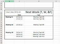
I want to break these meeting out into 3 views shown below called Today View, This Week View, and Next Week View.

The Example below is a table on Sheet2 and is the Today View. I have this one working fine.

C2 has the TODAY() function in it and based on what day it will show whatever meetings are occurring.
Thanks to some help that I received from this board.

C4 has the formula =IFERROR(FILTER(Sheet1!$B$3:$B$14,Sheet1!$B$3:$B$14=$C$2), "") and
D4 has =IFERROR(FILTER(Sheet1!$E$3:$E$14,Sheet1!$B$3:$B$14=$C$2),"")

on down the sheet.

The problem I am having is the "This week View" and the "Next Week View"

The above formulas does not work because I want all meetings in Meeting #1, Meeting #2, and Meeting #3 to be viewed at the same time.
The function =TODAY() only allows me to show what meetings are occurring that day.
I need a formula that would show all meetings for the current week.
You might be viewing on Friday of the current week but you see the meetings that already occurred that Tues and Wed and those that are occurring Friday.

I have the same problem with the "Next Week" View. I believe the formulas would be very similar.
I need a formula that would show all meetings for the Next week.

Thank you,
Ozz

 

[jasonb75]

The above formulas does not work because I want all meetings in Meeting #1, Meeting #2, and Meeting #3 to be viewed at the same time.
The function =TODAY() only allows me to show what meetings are occurring that day.

It may work if you use weekday to roll the date back to monday, then add 4 days to get to friday using both dates as min and max criteria. I can't test the theory on screen captures and don't have time to retype your sheets. I've used LET to simplify things a bit as the formulas will be quite messy. I've also taken the liberty of applying the same logic to your TODAY formula, this one should spill to both columns so will only need to be entered into one cell to fill the whole result range.

For meeting #1

Today

=LET(f,FILTER(Sheet1!$B$3:$E$14,{1,0,0,1}),c,FILTER(f,{1,0}),FILTER(f,c=C2,""))

This week

=LET(f,FILTER(Sheet1!$B$3:$E$14,{1,0,0,1}),c,FILTER(f,{1,0}),d,(C2-WEEKDAY(C2,3)),FILTER(f,(c>=d)+(c<=(d+4)),""))

Next week

=LET(f,FILTER(Sheet1!$B$3:$E$14,{1,0,0,1}),c,FILTER(f,{1,0}),d,(C2-WEEKDAY(C2,3)),FILTER(f,(c>=(d+7))+(c<=(d+11)),""))

For meeting #2, change the first array constant in each formula from {1,0,0,1} to {0,1,0,1}
For meeting #3, change them to {0,0,1,1}

Hopefully I haven't missed any parentheses this time

Edit:- as always, I re-read the question after posting and found some details that I overlooked straight away. Whilst the formulas that I've posted should work as required, I should be able to further simplify them, I'll take another look in the morning with fresh eyes in case there is something else that I haven't noticed yet.

 

[ozzborn]

Thank you, I will take a look in the morning. What you have done was what I was thinking. However, I do not have enough experience to figure the formula.

If I understand your formula ....the way it works I might be able to just use This Week and Next Week to deliver the same info.

Sometimes, my leadership likes information presented super simple. So that was the reason for the Today Table.

Unfortunatly the L2BB extension is not allowed on my work network.

Thanks will play with this in the morning.

Ozz

 

[jasonb75]

Leaving it until morning didn't happen for me, I started looking at other things, then went back to it and came up with this. I haven't filled in everything around it, but it is set up as per your original sheet (for the source and the results) with the exception of the dates in C2, etc being fixed rather than using TODAY() so that it matched your example for testing purposes.

Note that all formulas are dynamic arrays, 2 of them appear as normal formulas in the mini sheet below because there is no data to spill based on the current source so they are only populating a single cell.

ozzborn.xlsx
	B	C	D
2		18-Oct	Today
3		Date	Topic
4	Meeting #1	18-Oct-22	Meeting Topic #1
5		18-Oct-22	Meeting Topic #2
6		18-Oct-22	Meeting Topic #10
7		18-Oct-22	Meeting Topic #11
8	Meeting #2
9
10
11
12	Meeting #3
13
14
15
16
17
18		18-Oct	This week
19		Date	Topic
20	Meeting #1	18-Oct-22	Meeting Topic #1
21		18-Oct-22	Meeting Topic #2
22		18-Oct-22	Meeting Topic #10
23		18-Oct-22	Meeting Topic #11
24	Meeting #2	19-Oct-22	Meeting Topic #8
25
26
27
28	Meeting #3	21-Oct-22	Meeting Topic #8
29
30
31
32
33		18-Oct	This week
34		Date	Topic
35	Meeting #1	25-Oct-22	Meeting Topic #3
36		25-Oct-22	Meeting Topic #4
37
38
39	Meeting #2	26-Oct-22	Meeting Topic #9
40		26-Oct-22	Meeting Topic #11
41
42
43	Meeting #3	28-Oct-22	Meeting Topic #9
44		28-Oct-22	Meeting Topic #10
45		28-Oct-22	Meeting Topic #11
46
Sheet2

Cell Formulas
Range	Formula
C4:D7	C4	=LET(f,FILTER(Sheet1!$B$3:$E$14,{1,0,0,1}),FILTER(f,FILTER(f,{1,0})=C2,""))
C8	C8	=LET(f,FILTER(Sheet1!$B$3:$E$14,{0,1,0,1}),FILTER(f,FILTER(f,{1,0})=C2,""))
C12	C12	=LET(f,FILTER(Sheet1!$B$3:$E$14,{0,0,1,1}),FILTER(f,FILTER(f,{1,0})=C2,""))
C20:D23	C20	=LET(f,FILTER(Sheet1!$B$3:$E$14,{1,0,0,1}),FILTER(f,(FILTER(f,{1,0})=(C2-WEEKDAY(C2,3)+1)),""))
C24:D24	C24	=LET(f,FILTER(Sheet1!$B$3:$E$14,{0,1,0,1}),FILTER(f,(FILTER(f,{1,0})=(C2-WEEKDAY(C2,3)+2)),""))
C28:D28	C28	=LET(f,FILTER(Sheet1!$B$3:$E$14,{0,0,1,1}),FILTER(f,(FILTER(f,{1,0})=(C2-WEEKDAY(C2,3)+4)),""))
C35:D36	C35	=LET(f,FILTER(Sheet1!$B$3:$E$14,{1,0,0,1}),FILTER(f,(FILTER(f,{1,0})=(C2-WEEKDAY(C2,3)+8)),""))
C39:D40	C39	=LET(f,FILTER(Sheet1!$B$3:$E$14,{0,1,0,1}),FILTER(f,(FILTER(f,{1,0})=(C2-WEEKDAY(C2,3)+9)),""))
C43:D45	C43	=LET(f,FILTER(Sheet1!$B$3:$E$14,{0,0,1,1}),FILTER(f,(FILTER(f,{1,0})=(C2-WEEKDAY(C2,3)+11)),""))
Dynamic array formulas.

 

[ozzborn]

Thank you this looks real good. I do not think I will get to it today. I was pulled off this and put on another issue.
I hope to revisit it tomorrow.

 

[ozzborn]

Jasonb75, that worked perfect.

Thank you,
Ozz