Filtering Data Using not Exact Match

[TerrorTot38]

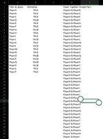
I am trying to extract / filter a list of names based on if a player is attending. For example if Player A is FALSE(not playing) only show the last 3 pairs highlighted in the example below.

I have a list of names of players. Column A (Players) Column B (Attending T / F)

- Player A - FALSE
- Player B - TRUE
- Player C - TRUE
- Player D - TRUE

I then have a list of pairs for example. Column D (Pairs not played)

- Player A & Player B
- Player A & Player C
- Player A & Player D
- Player B & Player C
- Player B & Player D
- Player C & Player D

Thus far I have

=VLOOKUP("*"&J2&"*",$M$2:$M$104,1,FALSE)

For example Kim and Kimberley are 2 different values.

Any ideas?

 

[StephenCrump]

Welcome to the Forum!

Here's one way:

	A	B	C	D	E	F	G	H
1	Player	Attending?		All			Filtered
2	A	TRUE		A	B		A	B
3	B	TRUE		A	C		A	D
4	C	FALSE		A	D		A	G
5	D	TRUE		A	E		A	H
6	E	FALSE		A	F		B	D
7	F	FALSE		A	G		B	G
8	G	TRUE		A	H		B	H
9	H	TRUE		B	C		D	G
10				B	D		D	H
11				B	E		G	H
12				B	F
13				B	G
14				B	H
15				C	D
16				C	E
17				C	F
18				C	G
19				C	H
20				D	E
21				D	F
22				D	G
23				D	H
24				E	F
25				E	G
26				E	H
27				F	G
28				F	H
29				G	H
30
Sheet1

Cell Formulas
Range	Formula
G2:H11	G2	=FILTER(All,MMULT(--VLOOKUP(All,Attending,2),SEQUENCE(2,,,0))=2,"No pairs!")
Dynamic array formulas.

Named Ranges
Name	Refers To	Cells
All	=Sheet1!$D$2:$E$29	G2
Attending	=Sheet1!$A$2:$B$9	G2

 

[TerrorTot38]

Thank you very much for the help on this. To get the data in column D & E. Did you manually extract the data?

If so if there a way to do this automatically using a formula as this would be perfect? I assuming you would use split on & or something similar?

 

[Peter_SSs]

Using the original layout, try this

22 02 03.xlsm
	A	B	C	D	E	F
1	Player	Attending?		All		Filtered
2	A	TRUE		A & B		A & B
3	B	TRUE		A & C		A & D
4	C	FALSE		A & D		A & G
5	D	TRUE		A & E		A & H
6	E	FALSE		A & F		B & D
7	F	FALSE		A & G		B & G
8	G	TRUE		A & H		B & H
9	H	TRUE		B & C		D & G
10				B & D		D & H
11				B & E		G & H
12				B & F
13				B & G
14				B & H
15				C & D
16				C & E
17				C & F
18				C & G
19				C & H
20				D & E
21				D & F
22				D & G
23				D & H
24				E & F
25				E & G
26				E & H
27				F & G
28				F & H
29				G & H
30
Filter Players

Cell Formulas
Range	Formula
F2:F11	F2	=LET(All,D2:D29,Attend,A2:B9,pos,FIND("&",All),FILTER(All,VLOOKUP(LEFT(All,pos-2),Attend,2,0)*VLOOKUP(REPLACE(All,1,pos+1,""),Attend,2,0),"No pairs"))
Dynamic array formulas.

 

[StephenCrump]

To get the data in column D & E. Did you manually extract the data?

I used a VBA function:

D2: =INDEX(Attending,GetCombinations(ROWS(Attending),2),1)

where:

Function GetCombinations(lNumber As Long, lNoChosen As Long) As Long()

    Dim lOutput() As Long, lCombinations As Long
    Dim i As Long, j As Long, k As Long
    
    lCombinations = WorksheetFunction.Combin(lNumber, lNoChosen)
    ReDim lOutput(1 To lCombinations, 1 To lNoChosen)
    
    For i = 1 To lNoChosen
        lOutput(1, i) = i
    Next i
    
    For i = 2 To lCombinations
        For j = 1 To lNoChosen
            lOutput(i, j) = lOutput(i - 1, j)
        Next j
        For j = lNoChosen To 1 Step -1
            lOutput(i, j) = lOutput(i, j) + 1
            If lOutput(i, j) <= lNumber - (lNoChosen - j) Then Exit For
        Next j
        For k = j + 1 To lNoChosen
            lOutput(i, k) = lOutput(i, k - 1) + 1
        Next k
    Next i
    
    GetCombinations = lOutput
    
End Function

 

[TerrorTot38]

Using the original layout, try this

22 02 03.xlsm
	A	B	C	D	E	F
1	Player	Attending?		All		Filtered
2	A	TRUE		A & B		A & B
3	B	TRUE		A & C		A & D
4	C	FALSE		A & D		A & G
5	D	TRUE		A & E		A & H
6	E	FALSE		A & F		B & D
7	F	FALSE		A & G		B & G
8	G	TRUE		A & H		B & H
9	H	TRUE		B & C		D & G
10				B & D		D & H
11				B & E		G & H
12				B & F
13				B & G
14				B & H
15				C & D
16				C & E
17				C & F
18				C & G
19				C & H
20				D & E
21				D & F
22				D & G
23				D & H
24				E & F
25				E & G
26				E & H
27				F & G
28				F & H
29				G & H
30
Filter Players

Cell Formulas
Range	Formula
F2:F11	F2	=LET(All,D2:D29,Attend,A2:B9,pos,FIND("&",All),FILTER(All,VLOOKUP(LEFT(All,pos-2),Attend,2,0)*VLOOKUP(REPLACE(All,1,pos+1,""),Attend,2,0),"No pairs"))
Dynamic array formulas.

Hi, I have tried copying this into F2 however my output is this:

Player	Attending		All		Filtered
A	TRUE​		A & B		#VALUE!​
B	TRUE​		A & C		#N/A​
C	FALSE​		A & D		#N/A​
D	TRUE​		A & E		#N/A​
E	FALSE​		A & F		#N/A​
F	FALSE​		A & G		#N/A​
G	TRUE​		A & H		#N/A​
H	TRUE​		B & C		#N/A​
			B & D		#N/A​

Any ideas why this could be?

 

[Peter_SSs]

Any ideas why this could be?

Yes, I would say that your TRUE/FALSE values in column B are text values not logical values. Try this instead.

22 02 03.xlsm
	A	B	C	D	E	F
1	Player	Attending?		All		Filtered
2	A	TRUE		A & B		A & B
3	B	TRUE		A & C		A & D
4	C	FALSE		A & D		A & G
5	D	TRUE		A & E		A & H
6	E	FALSE		A & F		B & D
7	F	FALSE		A & G		B & G
8	G	TRUE		A & H		B & H
9	H	TRUE		B & C		D & G
10				B & D		D & H
11				B & E		G & H
12				B & F
13				B & G
14				B & H
15				C & D
16				C & E
17				C & F
18				C & G
19				C & H
20				D & E
21				D & F
22				D & G
23				D & H
24				E & F
25				E & G
26				E & H
27				F & G
28				F & H
29				G & H
Filter Players (2)

Cell Formulas
Range	Formula
F2:F11	F2	=LET(All,D2:D29,Attend,A2:B9,pos,FIND("&",All),FILTER(All,(VLOOKUP(LEFT(All,pos-2),Attend,2,0)="TRUE")*(VLOOKUP(REPLACE(All,1,pos+1,""),Attend,2,0)="TRUE"),"No pairs"))
Dynamic array formulas.

 

[TerrorTot38]

Yes, I would say that your TRUE/FALSE values in column B are text values not logical values. Try this instead.

22 02 03.xlsm
	A	B	C	D	E	F
1	Player	Attending?		All		Filtered
2	A	TRUE		A & B		A & B
3	B	TRUE		A & C		A & D
4	C	FALSE		A & D		A & G
5	D	TRUE		A & E		A & H
6	E	FALSE		A & F		B & D
7	F	FALSE		A & G		B & G
8	G	TRUE		A & H		B & H
9	H	TRUE		B & C		D & G
10				B & D		D & H
11				B & E		G & H
12				B & F
13				B & G
14				B & H
15				C & D
16				C & E
17				C & F
18				C & G
19				C & H
20				D & E
21				D & F
22				D & G
23				D & H
24				E & F
25				E & G
26				E & H
27				F & G
28				F & H
29				G & H
Filter Players (2)

Cell Formulas
Range	Formula
F2:F11	F2	=LET(All,D2:D29,Attend,A2:B9,pos,FIND("&",All),FILTER(All,(VLOOKUP(LEFT(All,pos-2),Attend,2,0)="TRUE")*(VLOOKUP(REPLACE(All,1,pos+1,""),Attend,2,0)="TRUE"),"No pairs"))
Dynamic array formulas.

When I've copied this formula I now see No pairs as shown below:

Player	Attending		All		Filtered
A	TRUE​		A & B		No pairs
B	TRUE​		A & C
C	FALSE​		A & D
D	TRUE​		A & E
E	FALSE​		A & F
F	FALSE​		A & G
G	TRUE​		A & H
H	TRUE​		B & C
			B & D
			B & E
			B & F
			B & G
			B & H
			C & D
			C & E
			C & F
			C & G
			C & H
			D & E
			D & F
			D & G
			D & H
			E & F
			E & G
			E & H
			F & G
			F & H
			G & H

Thanks again

 

[StephenCrump]

Perhaps you're copying piece-meal? Did you know that with XL2BB you can copy the entire screenshot by clicking as indicated:

 

[TerrorTot38]

Perhaps you're copying piece-meal? Did you know that with XL2BB you can copy the entire screenshot by clicking as indicated:

View attachment 56877

Unfortunately my version of Office doesn't support BB2XL. As I have just tried to copy the data as one but just copies a HTML link.

However using one of your answers above and ensure all data in the table was filled out. That answer works but the one after it doesn't for some reason. I have marked it as the solution.

Thanks you very much for all your help again