Filtering One Condition to Multiple Columns on a Drop Down List

[pineapple61]

Hi everyone,

I have three columns A, B, and C and I want to filter the rows that pertain to one of the drop-down list selections that I created, what would be the formula for this?

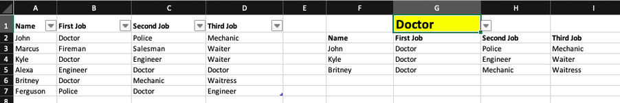
For example, I have listed the first, second and third job preferences of a number of people. I would like to see the names of the people that want to be a "doctor", no matter if it's their first, second or third preference. I have named my table "Work" to make it easier to filter and used the formula: =FILTER(Work, Work[First Job]=G1) - See image.

Now that I have filtered this and by using the selection list that I have, I can see the name of those that have Doctor as their first preference but I don't know how to add everyone else that has "Doctor" in their second and third job preference. What would be the formula for this?

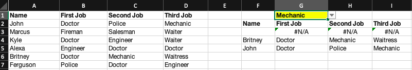
I tried to do this next but it did not work for me, =FILTER(Work, Work[First Job]=G1)*(Work[Second Job]=G1)

 

[Alex Blakenburg]

Thank you for including your version details in your profile and welcome to the Forum.

See if this works for you.

20230201 VStack Filter pineapple61.xlsx
	A	B	C	D	E	F	G	H	I
1	Name	First Job	Second Job	Third Job			Doctor
2	John	Doctor	Police	Mechanic		Name	First Job	Second Job	Third Job
3	Marcus	Fireman	Salesman	Waiter		John	Doctor	Police	Mechanic
4	Kyle	Doctor	Engineer	Waiter		Kyle	Doctor	Engineer	Waiter
5	Alexa	Engineer	Doctor	Doctor		Britney	Doctor	Mechanic	Waitress
6	Britney	Doctor	Mechanic	Waitress		Alexa	Engineer	Doctor	Doctor
7	Ferguson	Police	Doctor	Engineer		Ferguson	Police	Doctor	Engineer
Data

Cell Formulas
Range	Formula
F3:I7	F3	=UNIQUE(VSTACK(FILTER($A$2:$D$7,$B$2:$B$7=G1,""),FILTER($A$2:$D$7,$C$2:$C$7=G1,""),FILTER($A$2:$D$7,$D$2:$D$7=G1,"")))
Dynamic array formulas.

 

[pineapple61]

Thank you for including your version details in your profile and welcome to the Forum.

See if this works for you.

20230201 VStack Filter pineapple61.xlsx
	A	B	C	D	E	F	G	H	I
1	Name	First Job	Second Job	Third Job			Doctor
2	John	Doctor	Police	Mechanic		Name	First Job	Second Job	Third Job
3	Marcus	Fireman	Salesman	Waiter		John	Doctor	Police	Mechanic
4	Kyle	Doctor	Engineer	Waiter		Kyle	Doctor	Engineer	Waiter
5	Alexa	Engineer	Doctor	Doctor		Britney	Doctor	Mechanic	Waitress
6	Britney	Doctor	Mechanic	Waitress		Alexa	Engineer	Doctor	Doctor
7	Ferguson	Police	Doctor	Engineer		Ferguson	Police	Doctor	Engineer
Data

Cell Formulas
Range	Formula
F3:I7	F3	=UNIQUE(VSTACK(FILTER($A$2:$D$7,$B$2:$B$7=G1,""),FILTER($A$2:$D$7,$C$2:$C$7=G1,""),FILTER($A$2:$D$7,$D$2:$D$7=G1,"")))
Dynamic array formulas.

Thank you for including your version details in your profile and welcome to the Forum.

See if this works for you.

20230201 VStack Filter pineapple61.xlsx
	A	B	C	D	E	F	G	H	I
1	Name	First Job	Second Job	Third Job			Doctor
2	John	Doctor	Police	Mechanic		Name	First Job	Second Job	Third Job
3	Marcus	Fireman	Salesman	Waiter		John	Doctor	Police	Mechanic
4	Kyle	Doctor	Engineer	Waiter		Kyle	Doctor	Engineer	Waiter
5	Alexa	Engineer	Doctor	Doctor		Britney	Doctor	Mechanic	Waitress
6	Britney	Doctor	Mechanic	Waitress		Alexa	Engineer	Doctor	Doctor
7	Ferguson	Police	Doctor	Engineer		Ferguson	Police	Doctor	Engineer
Data

Cell Formulas
Range	Formula
F3:I7	F3	=UNIQUE(VSTACK(FILTER($A$2:$D$7,$B$2:$B$7=G1,""),FILTER($A$2:$D$7,$C$2:$C$7=G1,""),FILTER($A$2:$D$7,$D$2:$D$7=G1,"")))
Dynamic array formulas.

Wow, thanks! This is amazing, I've been struggling so much to get here. I have a quick question. If I select another job, e.g., "Mechanic", why are there cells that appear #N/A?

 

[Alex Blakenburg]

You can get rid of the NAs by including the IFNA or IFERROR function but unfortunately that left you with a blank row.
So it morphed into the below which should work as long as you don't put any numbers in Column 1 / A.

=LET(
fltrResult1,FILTER($A$2:$D$7, $B$2:$B$7=G1, 1),
fltrResult2,FILTER($A$2:$D$7, $C$2:$C$7=G1, 1),
fltrResult3,FILTER($A$2:$D$7, $D$2:$D$7=G1, 1),
vsResult,UNIQUE(VSTACK( fltrResult1, fltrResult2, fltrResult3 )),
vsResultCntThe1s,COUNT(CHOOSECOLS( vsResult, 1 )),
SORT(DROP( vsResult,  vsResultCntThe1s ), 1))

 

[pineapple61]

Awesome, it worked! One last question, I promise. This has helped me a lot, what would be the formula for the Microsoft Office Professional Plus 2016 version? Apparently, the FILTER option is not valid for that version, I think?

 

[Alex Blakenburg]

Can you ask that in a new thread. I don't know how to do it without using the dynamic array functions and you are more likely that someone fresh will look at it in a new thread. Just make it clear that it is question about converting the above to 2016 in the subject line and question, so that it is not viewed as being the same question duplicated.

Can you instal XL2BB ? You will more likely get a response if you provide an XL2BB so that helpers don't need to manually set up test data.
If you can't either paste some data in table form into your question or if need be provide a link to my post #2

XL2BB
MrExcel has a tool called “XL2BB” that lets you post samples of your data that will allow us to copy/paste it to our Excel spreadsheets, so we can work with the same copy of data that you are. Instructions on using this tool can be found here: XL2BB Add-in

Note that there is also a "Test Here” forum on this board. This is a place where you can test using this tool (or any other posting techniques that you want to test) before trying to use those tools in your actual posts.

 

[pineapple61]

Thanks for all the info, you have no idea how much I appreciate it!

 

[Alex Blakenburg]

You're welcome. Happy to help.