Knockoutpie
Board Regular
- Joined
- Sep 10, 2018
- Messages
- 116
- Office Version
- 365
- Platform
- Windows
a few weeks ago @DanteAmor helped me with some code which would find "partnum" in a row on sheet Quote, select that value and search for it in sheet "export", if found it would offset by 24 columns and select the value..
It works very well, exactly what I needed!
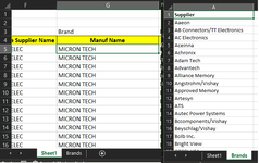
I'm trying to modify the code to find "brand" in row 3, on sheet1, move down 2 rows, select the value, and search for that value in column A in sheet "brands", if not found, highlight (in yellow) that selected value in Sheet1, and repeat until the end. I've modified it a little, and so far if it finds the result it changed it to "false" I get that it's a little redundant though and can be cut in half since i'm not offsetting or replacing values, just trying to highlight.
Maybe it would be easier to say if found, highlight in green? Because so far if it finds the value it replaced it with "false" so i'm half way there..
It works very well, exactly what I needed!
VBA Code:
Sub test_Dam()
Dim sh1 As Worksheet, sh2 As Worksheet
Dim f As Range
Dim i As Long, col1 As Long, col2 As Long, ini As Long

'set worksheet
Set sh1 = Sheets("Quote")
Set sh2 = Sheets("Export")

Set f = sh1.Cells.Find("Brand", , xlValues, xlPart, , , False)
If Not f Is Nothing Then
col1 = f.Column
ini = f.Row + 2
Set f = sh1.Cells.Find("Leadtime", , xlValues, xlPart, , , False)
If Not f Is Nothing Then
col2 = f.Column
For i = ini To sh1.Cells(Rows.Count, col1).End(3).Row
Set f = sh2.Cells.Find(sh1.Cells(i, col1).Value, , xlFormulas, xlPart, xlByRows, xlNext, False)
If Not f Is Nothing Then
sh1.Cells(i, col2).Value = f.Offset(0, 24).Value
End If
Next
End If
End If
End Sub
I'm trying to modify the code to find "brand" in row 3, on sheet1, move down 2 rows, select the value, and search for that value in column A in sheet "brands", if not found, highlight (in yellow) that selected value in Sheet1, and repeat until the end. I've modified it a little, and so far if it finds the result it changed it to "false" I get that it's a little redundant though and can be cut in half since i'm not offsetting or replacing values, just trying to highlight.
Maybe it would be easier to say if found, highlight in green? Because so far if it finds the value it replaced it with "false" so i'm half way there..
VBA Code:
       Sub Macro3()
'
' Macro3 Macro
'
Dim sh1 As Worksheet, sh2 As Worksheet
Dim f As Range
Dim i As Long, col1 As Long, col2 As Long, ini As Long

'set worksheet
Set sh1 = Sheets("Sheet1")
Set sh2 = Sheets("Brands")

' Pull Leadtime
Set a1 = sh1.Cells.Find("Brand", , xlValues, xlPart, , , False) ' Find Brand
If Not a1 Is Nothing Then
col1 = a1.Column
ini = a1.Row + 2
Set a1 = sh1.Cells.Find("Brand", , xlValues, xlPart, , , False) ' Find Brand ' is this needed since i'm not offsetting to another column?
If Not a1 Is Nothing Then
col2 = a1.Column
For a2 = ini To sh1.Cells(Rows.Count, col1).End(3).Row
Set a1 = sh2.Cells.Find(sh1.Cells(a2, col1).Value, , xlFormulas, xlPart, xlByRows, xlNext, False)
If Not a1 Is Nothing Then
sh1.Cells(a2, col2).Value = a1.Interior.Color = 5287936 ' Highlight isn't working, and changed the found value to 'false'
End If
Next
End If
End If
End Sub