Find first matching substring in a list and return adjacent value from another list

[chris32]

Hi there,

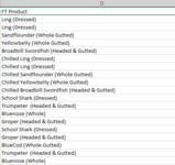
I am trying to find a way to harmonise the way a product is coded from various ways people may have entered it (i.e., the cut of fish - in parentheses here but note that this is not always the case).
For example, in the sample data below, "Gutted" and "whole gutted" mean the same thing, but "headed & gutted" is a different thing, and "whole" alone is yet a different thing.

TAB "Raw data", column A:

I am trying to automate the translation of these multiple possible terms people may use into a standard state code, by means of a formula in column B.
I have created a list of possible ways to name various cuts of fish (i.e. StateName) in a different tab "States translation" (column A), and the corresponding standard code (StateCode) next to it (column B).

TAB "States translation", column C and D:

I have made these two lists into arrays that I have named "StateName" and "StateCode" and that I would like to refer to in the tab where my raw data will be.
As you see in the two columns above, different states may include the same terms (e.g., gutted is found in GGT, GHCO, HGT and HGU) and so I have organised my list of possible terms in a hierarchical order, so that the search should end when the first matching StateName is found withing the string in column D.

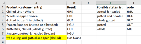
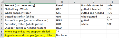
So for example, for the fifth term in column A, "Broadbill Swordfish (Headed & Gutted)", I'd like the formula to return HGU (rather than any of the codes above).

I have tried various methods (lookup, index, match) unsuccessfully as they either find multiple matches or result in lists of the same length as my arrays.

I have a very manual and inelegant solution to this problem, using IFS, ISNUMBER and SEARCH, but I am sure there must be a much more straightforward way than this:

=IF(D2<>"",IFS(ISNUMBER(SEARCH('States translation'!$C$2,D2)),'States translation'!$D$2,ISNUMBER(SEARCH('States translation'!$C$3,D2)),'States translation'!$D$3,ISNUMBER(SEARCH('States translation'!$C$4,D2)),'States translation'!$D$4,ISNUMBER(SEARCH('States translation'!$C$5,D2)),'States translation'!$D$5, [repeat same arguments with the entire list of 180+ items ] , TRUE,"Check"),"")

Many thanks for your help!

PS: Note that more state names could always be added to my arrays later on if it turn out that people have used names that were not covered in my current lists.

 

[chris32]

The $ signs that you added in from of the column letters will not hurt, but were not needed. Since the formula is being dragged down (not across) it is only the row numbers that need anchoring with $ signs and my formula already had $ signs before the row numbers. All you really needed to do was increase the 83 to 200.

Ah yes, got you! Thank you.

We could accommodate that with
Excel Formula:
=IFNA(VLOOKUP(REPLACE(LEFT(D2,LEN(D2)-1),1,FIND("(",D2),""),'States translation'!C$2:D$200,2,0),IFNA(VLOOKUP(REPLACE(LEFT(D2,LEN(D2)-2),1,FIND("(",D2),""),'States translation'!C$2:D$200,2,0),"Not Found"))

That does the trick perfectly!

chris32 said:
Is there a way to not rely on finding the parenthesis and independently searching for the substring?

I don't see how you could logically decide what part of a multi-word string is the substring to look for if there is nothing to identify it?

Hmm, I am not sure, I am not up to scratch with search functions! I have used the ISNUMBER(SEARCH()) combination with individual strings and it seems to be searching for the exact substring amongst the whole string without needing a starting point, like here:

=IF(D2<>"",IFS(ISNUMBER(SEARCH("chilled",D2)),"Chilled",ISNUMBER(SEARCH("frozen",D2)),"Frozen",TRUE,"Chilled"),"")

However, I have no idea if something like this could be used here where we need to search an entire list of possible terms instead of an individual search term - i.e., something like : ISNUMBER(SEARCH({StateName},D2) in which StarteName would be my list {"headed and gutted", "whole gutted", "gutted", "whole", ...}

PS: apologies, I had not yet seen your response when I sent the previous message.

 

[Peter_SSs]

the person entered "xxx ( whole gutted)" with an extra space after the parenthesis and so it did not find the matching state.

Just ignoring the parentheses wouldn't really help as the person may have accidentally inserted the extra space between 'whole' and 'gutted' instead and then the term still would not be found. However, still using the parentheses, we could eliminate any extra space problem with this.

=IFNA(VLOOKUP(TRIM(REPLACE(LEFT(D2,LEN(D2)-1),1,FIND("(",D2),"")),'States translation'!C$2:D$200,2,0),IFNA(VLOOKUP(TRIM(REPLACE(LEFT(D2,LEN(D2)-2),1,FIND("(",D2),"")),'States translation'!C$2:D$200,2,0),"Not Found"))

In relation to not using parentheses to locate the term, I don't think you understand the problem - or else I don't understand what you are saying.
Take this example
In B1 I am looking to return the value from column E that is associated with the substring in parentheses. Clearly the expected result is "C"

chris32.xlsm
	A	B	C	D	E
1	I am looking for a (particular term)			term	A
2				looking for	B
3				particular term	C
Sheet1

Now, consider this example that does not have the parentheses to identify the substring to search for.
What should we expect in B1 since it could be any of the three possibilities? And what is the logic to get the result?

chris32.xlsm
	A	B	C	D	E
1	I am looking for a particular term			term	A
2				looking for	B
3				particular term	C
Sheet1

 

[chris32]

In relation to not using parentheses to locate the term, I don't think you understand the problem - or else I don't understand what you are saying.

Now, consider this example that does not have the parentheses to identify the substring to search for.
What should we expect in B1 since it could be any of the three possibilities? And what is the logic to get the result?

Hi Peter,

thank you again for your help!
I understand the problem you mention now. I probably did not explain the data I am dealing with well enough, sorry about that!
The customer entries contain up to three types of information: the fish species (ling, snapper, butterfish, etc), the state (gutted, whole, etc) and most of the time the freshness (chilled vs. frozen). These three types of information can be input by the customer in any format (with or without parentheses around state or freshness) like in column A below:

I think the difficulty you mention of finding several matching terms in the costumer entries should not be an issue here, because the terms related to state (in yellow) should never overlap with terms related to species or freshness.

Terms that describe a state can overlap however, which is why I need to carefully order my list of possible states and have a search for exact matches, so that the formula finds the appropriate/shortest substring last (e.g., for "Chilled Ling - Whole", it should find the 5th state "whole" and not do a partial match on "whole gutted" for example, coming up with the wrong state).

Does it make more sense?

Thank you!

 

[chris32]

Hi all,

Just wanted to let you know that I have found a formula that works for me with the help of a colleague:

=XLOOKUP(TRUE,ISNUMBER(SEARCH('States translation'!B:B,J2)),'States translation'!C:C,"check"

Thank you for all the help!

 

[Peter_SSs]

Glad you have a solution but I have a few comments.

• I cannot see that formula ever returning "check". Doesn't it return 0 if no matches found?
• Best not to use whole column references like that. It is forcing Excel to check all 1 million+ rows in 'States translation' creating quite a calculation burden. Surely your list in 'States translation' is nothing like 1 million+ rows?
• Your profile says that you are using Excel 2019 - which does not have the XLOOKUP function. Have you changed versions?

BTW, the reason (or at least one reason) I was not having success for you was that I thought that you were looking to see if the substring in the 'Raw data' text appeared in the 'States translation' list but it appears that in fact you are looking to see if the 'States translation' list values appear in the 'Raw data' text.

 

[chris32]

Hi Peter,

you are right, the formula returns 0 rather than "check". Do you know why it might be?

Good point on the column reference. I have adapted the formula to search a specific array rather than the whole column.

My bad regarding the Excel version, I have checked and it is Excel 365. Hope that it did not send you on the wrong track with my problem! I have corrected the information in my profile.

Yes, I was looking to find states in the "States translation" list within the larger customer entry in the "Raw data". Sorry for not explaining that more clearly.

Many thanks for your help and many inputs.

 

[Peter_SSs]

you are right, the formula returns 0 rather than "check". Do you know why it might be?

Yes. Because the range (whole column) in 'States translation' contains blank cells, the SEARCH functions finds that at the beginning of all your J column cells so returns a 1, which meets the ISNUMBER() criteria. The "check" in that formula is returned only if ISNUMBER(SEARCH( fails for every row in the range - never going to happen with blanks in the range.

You could try this instead. Just check the range is big enough to accommodate the longest list you are likely to get in 'States translation'.

=INDEX(FILTER('States translation'!C$2:C$1000,ISNUMBER(SEARCH('States translation'!B$2:B$1000,J2))*('States translation'!B$2:B$1000<>""),"Check"),1)

 

[chris32]

You could try this instead. Just check the range is big enough to accommodate the longest list you are likely to get in 'States translation'.

=INDEX(FILTER('States translation'!C$2:C$1000,ISNUMBER(SEARCH('States translation'!B$2:B$1000,J2))*('States translation'!B$2:B$1000<>""),"Check"),1)

Hi Peter,

that makes sense. This version works perfectly! Many thanks for your help

 

[Peter_SSs]

You're welcome. Glad to contribute.