Find match of row header using a lookup

[pabybhoy]

Hi,

This may be diffult to explain so apologies in advance.
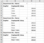
I'm creating a summary sheet which uses another file to lookup the salary and department using the surname. I can get the salary ok using vlookup but im having trouble getting the department due to the format of the sheet.
I need it to find the name (Col B) then move one cell right, search up to find next non blank cell then give me the cell value above that one.

Is this possible in a formula or even vba?
Unfortunately I can't change the format of this sheet as it come direct from the system, and it needs to be dynamic as the number of employees could change.
I've attached an example of lookup sheet.
Thanks

 

[Misca]

Looks like Power Query (or "Get & Transform" as they call it nowadays) would be your best friend here. It was first introduced as a free Excel addin in 2013 and has been found under the Data tab of the ribbon since Excel 2016.

You'll find great Power Query tutorials in YouTube. What you basically need is the "Fill down" option but you might as well want to get rid of the total rows & extra headers as well.

 

[Yongle]

or try this to see if it works for you

cells H2 and I2 make it easier to follow how the formula works

Do the whole thing in one formula using formula in J2
=INDEX(OFFSET(C1,0,0,MATCH(G2,B:B,0)),MAX((OFFSET(C1,0,0,MATCH(G2,B:B,0))<>"")*(ROW(OFFSET(C1,0,0,MATCH(G2,B:B,0))))))

Book1
	A	B	C	D	E	F	G	H	I	J	K
1	Department No. /Name		Apples	-			Name	Match row	Dept	In one
2	EmpRef	Employee Name		Salary			Shona	11	Oranges	Oranges
3		Peter		2503
4		John		2504
5		Mary		2505
6	Department No. /Name		Oranges	-
7	EmpRef	Employee Name		Salary
8		Harry		2508
9		Jenny		2509
10		Naomi		2510
11		Shona		2511
12	Department No. /Name		Pears	-
13	EmpRef	Employee Name		Salary
14		Graham		2514
15		Brian		2515
16		Lorna		2516
17		Charles		2517
18
Sheet1

Cell Formulas
Range	Formula
H2	H2	=MATCH(G2,B:B,0)
I2	I2	=INDEX(OFFSET(C1,0,0,H2),MAX((OFFSET(C1,0,0,H2)<>"")*(ROW(OFFSET(C1,0,0,H2)))))
J2	J2	=INDEX(OFFSET(C1,0,0,MATCH(G2,B:B,0)),MAX((OFFSET(C1,0,0,MATCH(G2,B:B,0))<>"")*(ROW(OFFSET(C1,0,0,MATCH(G2,B:B,0))))))

 

[pabybhoy]

or try this to see if it works for you

cells H2 and I2 make it easier to follow how the formula works

Do the whole thing in one formula using formula in J2
=INDEX(OFFSET(C1,0,0,MATCH(G2,B:B,0)),MAX((OFFSET(C1,0,0,MATCH(G2,B:B,0))<>"")*(ROW(OFFSET(C1,0,0,MATCH(G2,B:B,0))))))

Book1
	A	B	C	D	E	F	G	H	I	J	K
1	Department No. /Name		Apples	-			Name	Match row	Dept	In one
2	EmpRef	Employee Name		Salary			Shona	11	Oranges	Oranges
3		Peter		2503
4		John		2504
5		Mary		2505
6	Department No. /Name		Oranges	-
7	EmpRef	Employee Name		Salary
8		Harry		2508
9		Jenny		2509
10		Naomi		2510
11		Shona		2511
12	Department No. /Name		Pears	-
13	EmpRef	Employee Name		Salary
14		Graham		2514
15		Brian		2515
16		Lorna		2516
17		Charles		2517
18
Sheet1

Cell Formulas
Range	Formula
H2	H2	=MATCH(G2,B:B,0)
I2	I2	=INDEX(OFFSET(C1,0,0,H2),MAX((OFFSET(C1,0,0,H2)<>"")*(ROW(OFFSET(C1,0,0,H2)))))
J2	J2	=INDEX(OFFSET(C1,0,0,MATCH(G2,B:B,0)),MAX((OFFSET(C1,0,0,MATCH(G2,B:B,0))<>"")*(ROW(OFFSET(C1,0,0,MATCH(G2,B:B,0))))))

Hi,

Thanks for the reply. I've tested this formula and I'm getting the top line every time. Its getting the Match Row but formulas in col I & J both give "Apples"

Book33
	A	B	C	D	E	F	G	H	I	J
1	Department No. / Name :		Apples	-			Name	Match Row	Dept	In one
2	Emp Ref	Employee Name	salary				Cross	11	Apples	Apples
3		Smith		2500.00
4		Jones		2501.00
5		Parker		2502.00
6		Johnson		2503.00
7	Department No. / Name :		Oranges	-
8	Emp Ref	Employee Name	salary
9		Baker		2504.00
10		Martin		2501.00
11		Cross		2502.00
12		Dept. Total :		7507.00
13	Department No. / Name :		Pears	-
14	Emp Ref	Employee Name	salary
15		Ferguson		2500.00
16		Dept. Total :		2500.00
17
Sheet1

Cell Formulas
Range	Formula
H2	H2	=MATCH(G2,B:B,0)
I2	I2	=INDEX(OFFSET(C1,0,0,H2),MAX((OFFSET(C1,0,0,H2)<>"")*(ROW(OFFSET(C1,0,0,H2)))))
J2	J2	=INDEX(OFFSET(C1,0,0,MATCH(G2,B:B,0)),MAX((OFFSET(C1,0,0,MATCH(G2,B:B,0))<>"")*(ROW(OFFSET(C1,0,0,MATCH(G2,B:B,0))))))

 

[pabybhoy]

Ignore the above. I hadn't used the Control Shift to enter the formula.
I had to tweak slightly as the word salary is underneath the dept name but got it working now.
Thank you so much for all your help

 

[Yongle]

How strange that it works for me, but not for you
- everything looks identical

Something you could try which also works for me
- edit cell J2 and (instead of the usual ENTER ) confirm the formula with {CRTRL}{SHIFT}{ENTER}
- which converts the formula to an array formula and places { } around the formula (which does not work if you do it manually
- same for cell I2

 

[Yongle]

It may be an Excel 365 change - perhaps 365 recognises an array formula without being told explicitly

 

[pabybhoy]

It may be an Excel 365 change - perhaps 365 recognises an array formula without being told explicitly

Hi, See above your last post. It was the array formula. Got it working now. Thanks again for your help

 

[Yongle]