find multiple and repeating combinations

[danonanno]

Hi, all
Very new to this so go easy on me.
I have an excel file with many rows of data. Column B has store numbers and column C product id Numbers. For instance B1=210, B2=210. C1=27142,and C2=27143. This means that store 210 gets product id # 27142 and 27143. Simple huh. These 2 products will repeat throughout column B with different store numbers each time. The trick is to identify all the stores that get these 2 products. Now there is another twist. B3=211,B4=211,and B5=211. C3=12345,C4=12346,C5=27142. This means that store 211 gets products 12345,12346,27142. Notice that stores 210 and 211 both get product # 27142. These 3 products will also repeat throughout the file and the trick is to find all the stores that take these combinations of products. Probably an easy solution but when ya don"t know ya just don't know. Thanks for any help you can give me.

 

[Greg Truby]

Denis, I am not able to visualize how you can get what Danonanno wants using a pivot laid out like you describe.

Danonanno, I'm working on a post to explain "phase I" to you -- how to do it manually. Then w/ Phase II we can talk about using some VBA. And maybe a Phase III - VBA bells & whistles.

Back soon.

 

[Greg Truby]

I did try Dom's but I muffed up something and can't get it to work properly. Nonetheless, while it is some amazing formula-smithing I still think it would get really, really expensive in terms of calculation burdens. So here's the pivot thing -- manually. We get the first part done a understand that bit then we can see if a touch of VBA would make life easier.

Our sample data is as posted here but with column A having a header Store and column B having a header Prod ID.

Were this sans the combination bit, this would be a very simple pivot table. Just drag Store in as a row field and Prod ID as both the column field and the data field. By default we would get:

Post topic 231459.xls
	A	B	C	D	E
3	Count of Prod ID	Prod ID
4	Store	12345	12346	27142	27143
5	210			1	1
6	211	1	1	1
7	212			1	1
8	213	1	1	1
9	214	1	1	1
10	Grand Total	3	3	5	2
Simple Pivot

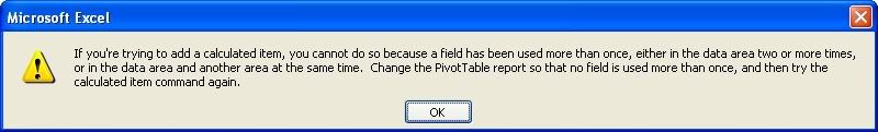
But we need calculated items. If we try to create calculated items with that pivot table, Excel is gonna whine at us:



So we need to create a dummy field. All we do is take column C, add in a header Dummy and fill the column with 1's.<table border="1" bordercolor="#C0C0C0" bordercolordark="#FFFFFF" cellspacing="0" align="left"><tr valign="top" style="white-space:nowrap;"><th width="63" height="21" valign="bottom"><font face="Monospace" size="1">Store</font></th><th width="63" height="21" valign="bottom"><font face="Monospace" size="1">Prod ID</font></th><th width="63" height="21" valign="bottom"><font face="Monospace" size="1">Dummy</font></th></tr><tr valign="top" style="white-space:nowrap;"><td width="63" height="21" align="right" valign="bottom"><font face="Monospace" size="1">210</font></td><td width="63" height="21" align="right" valign="bottom"><font face="Monospace" size="1">27142 </font></td><td width="63" height="21" align="right" valign="bottom"><font face="Monospace" size="1">1</font></td></tr><tr valign="top" style="white-space:nowrap;"><td width="63" height="21" align="right" valign="bottom"><font face="Monospace" size="1">210</font></td><td width="63" height="21" align="right" valign="bottom"><font face="Monospace" size="1">27143 </font></td><td width="63" height="21" align="right" valign="bottom"><font face="Monospace" size="1">1</font></td></tr><tr valign="top" style="white-space:nowrap;"><td width="63" height="21" align="right" valign="bottom"><font face="Monospace" size="1">211</font></td><td width="63" height="21" align="right" valign="bottom"><font face="Monospace" size="1">12345 </font></td><td width="63" height="21" align="right" valign="bottom"><font face="Monospace" size="1">1</font></td></tr><tr valign="top" style="white-space:nowrap;"><td width="63" height="21" align="right" valign="bottom"><font face="Monospace" size="1">211</font></td><td width="63" height="21" align="right" valign="bottom"><font face="Monospace" size="1">12346 </font></td><td width="63" height="21" align="right" valign="bottom"><font face="Monospace" size="1">1</font></td></tr><tr valign="top" style="white-space:nowrap;"><td width="63" height="21" align="right" valign="bottom"><font face="Monospace" size="1">211</font></td><td width="63" height="21" align="right" valign="bottom"><font face="Monospace" size="1">27142 </font></td><td width="63" height="21" align="right" valign="bottom"><font face="Monospace" size="1">1</font></td></tr><tr valign="top" style="white-space:nowrap;"><td width="63" height="21" align="right" valign="bottom"><font face="Monospace" size="1">212</font></td><td width="63" height="21" align="right" valign="bottom"><font face="Monospace" size="1">27142 </font></td><td width="63" height="21" align="right" valign="bottom"><font face="Monospace" size="1">1</font></td></tr><tr valign="top" style="white-space:nowrap;"><td width="63" height="21" align="right" valign="bottom"><font face="Monospace" size="1">212</font></td><td width="63" height="21" align="right" valign="bottom"><font face="Monospace" size="1">27143 </font></td><td width="63" height="21" align="right" valign="bottom"><font face="Monospace" size="1">1</font></td></tr><tr valign="top" style="white-space:nowrap;"><td width="63" height="21" align="right" valign="bottom"><font face="Monospace" size="1">213</font></td><td width="63" height="21" align="right" valign="bottom"><font face="Monospace" size="1">12345 </font></td><td width="63" height="21" align="right" valign="bottom"><font face="Monospace" size="1">1</font></td></tr><tr valign="top" style="white-space:nowrap;"><td width="63" height="21" align="right" valign="bottom"><font face="Monospace" size="1">213</font></td><td width="63" height="21" align="right" valign="bottom"><font face="Monospace" size="1">12346 </font></td><td width="63" height="21" align="right" valign="bottom"><font face="Monospace" size="1">1</font></td></tr><tr valign="top" style="white-space:nowrap;"><td width="63" height="21" align="right" valign="bottom"><font face="Monospace" size="1">213</font></td><td width="63" height="21" align="right" valign="bottom"><font face="Monospace" size="1">27142 </font></td><td width="63" height="21" align="right" valign="bottom"><font face="Monospace" size="1">1</font></td></tr><tr valign="top" style="white-space:nowrap;"><td width="63" height="21" align="right" valign="bottom"><font face="Monospace" size="1">214</font></td><td width="63" height="21" align="right" valign="bottom"><font face="Monospace" size="1">12345 </font></td><td width="63" height="21" align="right" valign="bottom"><font face="Monospace" size="1">1</font></td></tr><tr valign="top" style="white-space:nowrap;"><td width="63" height="21" align="right" valign="bottom"><font face="Monospace" size="1">214</font></td><td width="63" height="21" align="right" valign="bottom"><font face="Monospace" size="1">12346 </font></td><td width="63" height="21" align="right" valign="bottom"><font face="Monospace" size="1">1</font></td></tr><tr valign="top" style="white-space:nowrap;"><td width="63" height="21" align="right" valign="bottom"><font face="Monospace" size="1">214</font></td><td width="63" height="21" align="right" valign="bottom"><font face="Monospace" size="1">27142 </font></td><td width="63" height="21" align="right" valign="bottom"><font face="Monospace" size="1">1</font></td></tr></table>



You might need to use the wizard and backup to the 2^nd setup step and re-define the used area to include column C now. So we go back to our pivot, drag Prod ID out of the data area (grab cell A3 and drag it off the pivot to do this). Now drag dummy into the data area and you get this:

Post topic 231459.xls
	A	B	C	D	E
3	Sum of Dummy	Prod ID
4	Store	12345	12346	27142	27143
5	210			1	1
6	211	1	1	1
7	212			1	1
8	213	1	1	1
9	214	1	1	1
10	Grand Total	3	3	5	2
Simple Pivot (2)

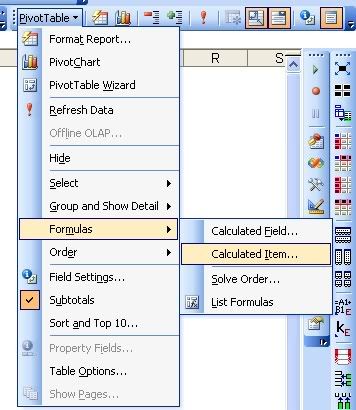
Select a cell with a product ID in it in the pivot, i.e. a cell in B4:E4 and then click on the pivot table toolbar to pull up the Formulas > | Calculated Item... menu option.



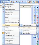
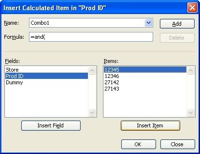
You should now see the Insert Calculated Item in "Prod ID" dialog box.



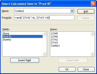
Type Combo1 in the Name box and then =and( in the Formula box. If Prod ID is not selected in the Fields list, select it. Then you can pick '12345' from the Items list and click the Insert Item button and then in the formula box add in >0, and then add the next item and so forth until you build the formula to be =AND('12345' >0,'12346' >0,'27142' >0)



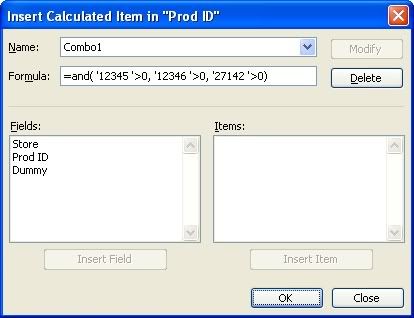
Repeat the process to define a second calculated item: Combo2



Click the OK button at the bottom and you should have what I posted earlier.

 

[Domenic]

I did try Dom's but I muffed up something and can't get it to work properly.

Since you've taken the time to try my solution, I'd be happy to send you a sample file, if you'd like.

...I still think it would get really, really expensive in terms of calculation burdens.

I haven't tried it on a large set of data, but it may very well be the case.

 

[erik.van.geit]

Yes, it will be expensive, especially when taking into acount.

This file has to be sorted 1 time per month

so waiting for response

Where will the different combos be located ?
And where do you want to get the results ? Separate sheet ? Layout ?

 

[danonanno]

thanks greg, I have phase 1 done ok

 

[Greg Truby]

Erik,

Rather than re-invent the functionality of the pivot w/ VBA, I'd say just use VBA to control a pivot and let the pivot do the heavy lifting. Would you be able to help danonanno put that together? I'm just not going to have time in the next couple of weeks. I've spent too much time on the boards today as it is...

Regards,

 

[erik.van.geit]

Hi, Greg,

Yes, I was thinking some hours ago, when does Greg doe all this stuff while he's at the office? (Currently I'm not in "need" to "work" a lot so I've spent quite some time on the Board)
But, the kind of applications I've built did never need PivotTables, so my experience is almost zero
The good news is, I'm quite sure this is easy coding, but I need to get some answers, danonanno, to questions which I already posted twice.

have a nice time!
Erik

 

[SydneyGeek]

Taking on board the most recent posts, here is a variation on the pivot table theme and some VBA.
At the moment the PT will need to be re-created by hand and named StorePivot, but that can easily be automated if this turns out to be useful.
Here is the sheet layout after creating the first pivot and running the code:

Book1
	A	B	C	D	E	F	G	H
1	Store	Product		Store	214		Store	ProductList
2	210	27142					210	27142;27143
3	210	27143		SumofProduct			211	12345;12346;27142
4	211	12345		Product	Total		212	27143
5	211	12346		12345	12345		213	12345;12346;27142
6	211	27142		12346	12346		214	12345;12346;27142
7	212	27143		27142	27142
8	212	27143
9	213	12345
10	213	12346
11	213	27142
12	214	12345
13	214	12346
14	214	27142
Sheet1

Here is the second pivot, to give a sorted list of all current product combos with the strores that stock them:

Book1
	J	K	L	M
4	ProductList	Store
5	27143	212
6	12345;12346;27142	211
7		213
8		214
9	27142;27143	210
10
Sheet1

Here is the VBA:

Sub RunPages()
    Dim PT As PivotTable
    Dim PField As PivotField
    Dim PItem As PivotItem
    Dim PList As PivotItemList
    Dim sText As String
    Dim i As Long
    Dim c As Range
    i = 2
    Set PT = ActiveSheet.PivotTables("StorePivot")
    Set PField = PT.PivotFields("Store")
    
    Application.ScreenUpdating = False
    For Each PItem In PField.PivotItems
        'select a store and refresh the table
        PField.CurrentPage = PItem.Value
        PT.ManualUpdate = True
        PT.ManualUpdate = False
        sText = ""
        Cells(i, 7) = PItem
        For Each c In Range(Cells(5, 4), Cells(65536, 4).End(xlUp))
            sText = sText & c.Value & ";"
        Next c
        sText = Left(sText, Len(sText) - 1)
        Cells(i, 8) = sText
        i = i + 1
    Next PItem
    Application.ScreenUpdating = True
End Sub

1. The first pivot places Store in the Page field, so you can filter for each store in turn. I ran a test with about 10K rows of random data (900 stores) and returned a list of about 1800 unique combinations in about 20 seconds.

2. The intermediate data has been left on the same sheet to illustrate the concept. This can be pushed to a temporary sheet that is deleted once the result is back on Sheet1

3. Both pivots are simple to create in VBA. It would be logical to do just that, so this becomes a one-step process.

Denis

 

[danonanno]

sorry eric, I thought one of your posts with a question was directed to one of the guys working on a solution. This has been extremely helpful and i want to thank all of you. I'm going to try a few of these things then would like to know more about writing code to automate the whole process. What a great bunch of guys. Thanks again!!!!!

 

[danonanno]

eric, sorry for the misunderstanding. the sample of the file i posted is all i get . I have to look at it to see what possible combinations of sku's there are. The output would be a list of stores that get each combo. It doesnt matter if this is all on one sheet or each combo on a different worksheet. The simpler the better. The pivot table ideas have been helpful. But would eventually like to code this to speed things up. Most files i get have about 6 different combo's of sku's. Have had up to 38 though. So far combo's have been between 1 and 7 sku's. Bottom line is , I need to learn more about coding. Hope i haven't caused more confusion. Thanks